

3.2 Ground-State Expectation Values
37
A ≡ (a rs )
(3.31)
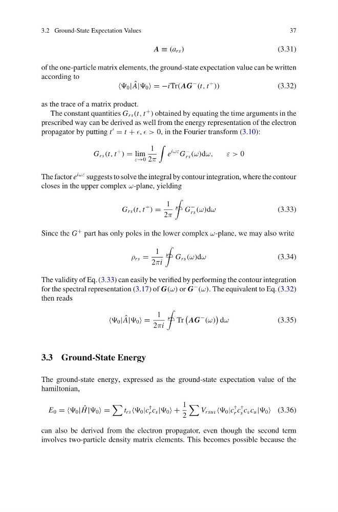
of the one-particle matrix elements, the ground-state expectation value can be written
according to
0 | ˆ
A| 0 = −iTr( AG
−
(t, t
+
))
(3.32)
as the trace of a matrix product.
The constant quantities G rs (t, t
+
) obtained by equating the time arguments in the
prescribed way can be derived as well from the energy representation of the electron
propagator by putting t
= t + , > 0, in the Fourier transform (3.10):
G rs (t, t
+
) = lim
ε→0
1
2π
e
iωε G
−
rs (ω)dω,
ε > 0
The factor e
iωε suggests to solve the integral by contour integration, where the contour
closes in the upper complex ω-plane, yielding
G rs (t, t
+
) =
1
2π
2 G
−
rs (ω)dω
(3.33)
Since the G
+ part has only poles in the lower complex ω-plane, we may also write
ρ rs =
1
2πi
2 G rs (ω)dω
(3.34)
The validity of Eq. (3.33) can easily be verified by performing the contour integration
for the spectral representation (3.17) of G(ω) or G
−
(ω). The equivalent to Eq. (3.32)
then reads
0 | ˆ
A| 0 =
1
2πi
2 Tr
AG
−
(ω)
dω
(3.35)
3.3 Ground-State Energy
The ground-state energy, expressed as the ground-state expectation value of the
hamiltonian,
E 0 = = 0 | ˆ
H | 0 =
t rs 0 |c
†
r c s | 0 +
1
2
V rsuv 0 |c
†
r c
†
s c v c u | 0 (3.36)
can also be derived from the electron propagator, even though the second term
involves two-particle density matrix elements. This becomes possible because the
37
A ≡ (a rs )
(3.31)
of the one-particle matrix elements, the ground-state expectation value can be written
according to
0 | ˆ
A| 0 = −iTr( AG
−
(t, t
+
))
(3.32)
as the trace of a matrix product.
The constant quantities G rs (t, t
+
) obtained by equating the time arguments in the
prescribed way can be derived as well from the energy representation of the electron
propagator by putting t
= t + , > 0, in the Fourier transform (3.10):
G rs (t, t
+
) = lim
ε→0
1
2π
e
iωε G
−
rs (ω)dω,
ε > 0
The factor e
iωε suggests to solve the integral by contour integration, where the contour
closes in the upper complex ω-plane, yielding
G rs (t, t
+
) =
1
2π
2 G
−
rs (ω)dω
(3.33)
Since the G
+ part has only poles in the lower complex ω-plane, we may also write
ρ rs =
1
2πi
2 G rs (ω)dω
(3.34)
The validity of Eq. (3.33) can easily be verified by performing the contour integration
for the spectral representation (3.17) of G(ω) or G
−
(ω). The equivalent to Eq. (3.32)
then reads
0 | ˆ
A| 0 =
1
2πi
2 Tr
AG
−
(ω)
dω
(3.35)
3.3 Ground-State Energy
The ground-state energy, expressed as the ground-state expectation value of the
hamiltonian,
E 0 = = 0 | ˆ
H | 0 =
t rs 0 |c
†
r c s | 0 +
1
2
V rsuv 0 |c
†
r c
†
s c v c u | 0 (3.36)
can also be derived from the electron propagator, even though the second term
involves two-particle density matrix elements. This becomes possible because the