

3.1 Definition and Relation to Physical Quantities
35
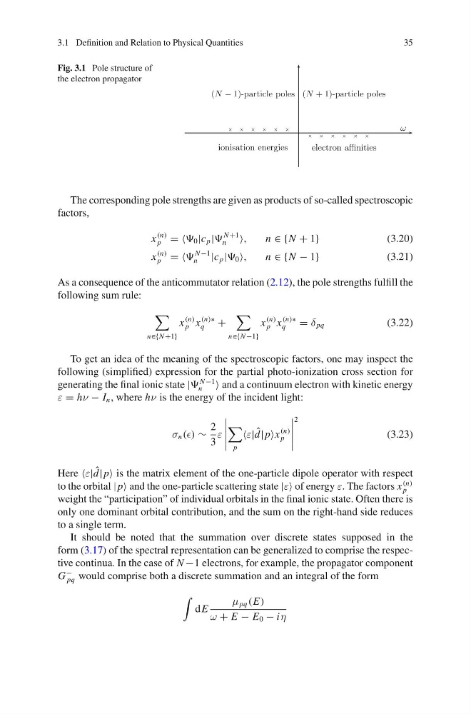
Fig. 3.1 Pole structure of
the electron propagator
The corresponding pole strengths are given as products of so-called spectroscopic
factors,
x
(n)
p = = 0 |c p |
N +1
n
,
n ∈ {N + 1}
(3.20)
x
(n)
p = =
N −1
n
|c p | 0 ,
n ∈ {N − 1}
(3.21)
As a consequence of the anticommutator relation (2.12), the pole strengths fulfill the
following sum rule:
n∈{N +1}
x
(n)
p x
(n)∗
q
+
n∈{N −1}
x
(n)
p x
(n)∗
q
= δ pq
(3.22)
To get an idea of the meaning of the spectroscopic factors, one may inspect the
following (simplified) expression for the partial photo-ionization cross section for
generating the final ionic state |
N −1
n
and a continuum electron with kinetic energy
ε = hν − I n , where hν is the energy of the incident light:
σ n () ∼
2
3
ε
p
ε| ˆ
d| px
(n)
p
2
(3.23)
Here ε| ˆ
d| p is the matrix element of the one-particle dipole operator with respect
to the orbital | p and the one-particle scattering state |ε of energy ε. The factors x
(n)
p
weight the “participation” of individual orbitals in the final ionic state. Often there is
only one dominant orbital contribution, and the sum on the right-hand side reduces
to a single term.
It should be noted that the summation over discrete states supposed in the
form (3.17) of the spectral representation can be generalized to comprise the respective continua. In the case of N −1 electrons, for example, the propagator component
G
−
pq would comprise both a discrete summation and an integral of the form
dE
μ pq (E)
ω + E − E 0 − iη
35
Fig. 3.1 Pole structure of
the electron propagator
The corresponding pole strengths are given as products of so-called spectroscopic
factors,
x
(n)
p = = 0 |c p |
N +1
n
,
n ∈ {N + 1}
(3.20)
x
(n)
p = =
N −1
n
|c p | 0 ,
n ∈ {N − 1}
(3.21)
As a consequence of the anticommutator relation (2.12), the pole strengths fulfill the
following sum rule:
n∈{N +1}
x
(n)
p x
(n)∗
q
+
n∈{N −1}
x
(n)
p x
(n)∗
q
= δ pq
(3.22)
To get an idea of the meaning of the spectroscopic factors, one may inspect the
following (simplified) expression for the partial photo-ionization cross section for
generating the final ionic state |
N −1
n
and a continuum electron with kinetic energy
ε = hν − I n , where hν is the energy of the incident light:
σ n () ∼
2
3
ε
p
ε| ˆ
d| px
(n)
p
2
(3.23)
Here ε| ˆ
d| p is the matrix element of the one-particle dipole operator with respect
to the orbital | p and the one-particle scattering state |ε of energy ε. The factors x
(n)
p
weight the “participation” of individual orbitals in the final ionic state. Often there is
only one dominant orbital contribution, and the sum on the right-hand side reduces
to a single term.
It should be noted that the summation over discrete states supposed in the
form (3.17) of the spectral representation can be generalized to comprise the respective continua. In the case of N −1 electrons, for example, the propagator component
G
−
pq would comprise both a discrete summation and an integral of the form
dE
μ pq (E)
ω + E − E 0 − iη