

34
3 One-Particle Green’s Function
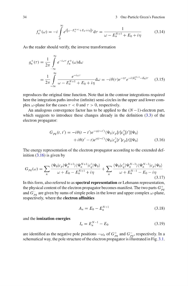
f
+
n (ω) = −i
∞
0
e
i[ω−E
N +1
n
+E 0 +iη]τ dτ =
1
ω − E
N +1
n
+ E 0 + iη
(3.14)
As the reader should verify, the inverse transformation
g
+
n (τ ) =
1
2π
∞
−∞
e
−iωτ f
+
n (ω)dω
=
1
2π
∞
−∞
e
−iωτ
ω − E
N +1
n
+ E 0 + iη
dω = −iθ(τ )e
−ητ e
−i(E
N +1
n
−E 0 )τ
(3.15)
reproduces the original time function. Note that in the contour integrations required
here the integration paths involve (infinite) semi-circles in the upper and lower complex ω-plane for the cases τ < 0 and τ > 0, respectively.
An analogous convergence factor has to be applied to the (N −1)-electron part,
which suggests to introduce these changes already in the definition (3.3) of the
electron propagator:
G pq (t, t
) = −iθ(t − t
)e
−η(t−t
)
0 |c p [t]c
†
q [t
]| 0
+ iθ(t
− t)e
η(t−t
)
0 |c
†
q [t
]c p [t]| 0
(3.16)
The energy representation of the electron propagator according to the extended definition (3.16) is given by
G pq (ω) =
n
0 |c p |
N +1
n
N +1
n
|c
†
q | 0
ω + E 0 − E
N +1
n
+ iη
+
n
0 |c
†
q |
N −1
n
N −1
n
|c p | 0
ω + E
N −1
n
− E 0 − iη
(3.17)
In this form, also referred to as spectral representation or Lehmann representation,
the physical content of the electron propagator becomes manifest. The two parts G
+
pq
and G
−
pq are given by sums of simple poles in the lower and upper complex ω-plane,
respectively, where the electron affinities
A n = E 0 − E
N +1
n
(3.18)
and the ionization energies
I n = E
N −1
n
− E 0
(3.19)
are identified as the negative pole positions −ω n of G
+
pq and G
−
pq , respectively. In a
schematical way, the pole structure of the electron propagator is illustrated in Fig. 3.1.
3 One-Particle Green’s Function
f
+
n (ω) = −i
∞
0
e
i[ω−E
N +1
n
+E 0 +iη]τ dτ =
1
ω − E
N +1
n
+ E 0 + iη
(3.14)
As the reader should verify, the inverse transformation
g
+
n (τ ) =
1
2π
∞
−∞
e
−iωτ f
+
n (ω)dω
=
1
2π
∞
−∞
e
−iωτ
ω − E
N +1
n
+ E 0 + iη
dω = −iθ(τ )e
−ητ e
−i(E
N +1
n
−E 0 )τ
(3.15)
reproduces the original time function. Note that in the contour integrations required
here the integration paths involve (infinite) semi-circles in the upper and lower complex ω-plane for the cases τ < 0 and τ > 0, respectively.
An analogous convergence factor has to be applied to the (N −1)-electron part,
which suggests to introduce these changes already in the definition (3.3) of the
electron propagator:
G pq (t, t
) = −iθ(t − t
)e
−η(t−t
)
0 |c p [t]c
†
q [t
]| 0
+ iθ(t
− t)e
η(t−t
)
0 |c
†
q [t
]c p [t]| 0
(3.16)
The energy representation of the electron propagator according to the extended definition (3.16) is given by
G pq (ω) =
n
0 |c p |
N +1
n
N +1
n
|c
†
q | 0
ω + E 0 − E
N +1
n
+ iη
+
n
0 |c
†
q |
N −1
n
N −1
n
|c p | 0
ω + E
N −1
n
− E 0 − iη
(3.17)
In this form, also referred to as spectral representation or Lehmann representation,
the physical content of the electron propagator becomes manifest. The two parts G
+
pq
and G
−
pq are given by sums of simple poles in the lower and upper complex ω-plane,
respectively, where the electron affinities
A n = E 0 − E
N +1
n
(3.18)
and the ionization energies
I n = E
N −1
n
− E 0
(3.19)
are identified as the negative pole positions −ω n of G
+
pq and G
−
pq , respectively. In a
schematical way, the pole structure of the electron propagator is illustrated in Fig. 3.1.