

3.1 Definition and Relation to Physical Quantities
33
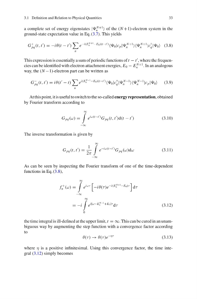
a complete set of energy eigenstates |
N +1
n
of the (N +1)-electron system in the
ground-state expectation value in Eq. (3.7). This yields
G
+
pq (t, t
) = −iθ(t − t
)
n
e
−i(E
N +1
n
−E 0 )(t−t
)
0 |c p |
N +1
n
N +1
n
|c
†
q | 0 (3.8)
This expression is essentially a sum of periodic functions of t − t
, where the frequencies can be identified with electron attachment energies, E 0 − E
N +1
n
. In an analogous
way, the (N −1)-electron part can be written as
G
−
pq (t, t
) = iθ(t
− t)
n
e
i(E
N −1
n
−E 0 )(t−t
)
0 |c
†
q |
N −1
n
N −1
n
|c p | 0 (3.9)
At this point, it is useful to switch to the so-called energy representation, obtained
by Fourier transform according to
G pq (ω) =
∞
−∞
e
iω(t−t
) G pq (t, t
)d(t − t
)
(3.10)
The inverse transformation is given by
G pq (t, t
) =
1
2π
∞
−∞
e
−iω(t−t
) G pq (ω)dω
(3.11)
As can be seen by inspecting the Fourier transform of one of the time-dependent
functions in Eq. (3.8),
f
+
n (ω) =
∞
−∞
e
iωτ
−iθ(τ )e
−i(E
N +1
n
−E 0 )τ
dτ
= −i
∞
0
e
i[ω−E
N +1
n
+E 0 ]τ dτ
(3.12)
the time integral is ill-defined at the upper limit, t = ∞. This can be cured in an unambiguous way by augmenting the step function with a convergence factor according
to
θ(τ ) → θ(τ )e
−ητ
(3.13)
where η is a positive infinitesimal. Using this convergence factor, the time integral (3.12) simply becomes
33
a complete set of energy eigenstates |
N +1
n
of the (N +1)-electron system in the
ground-state expectation value in Eq. (3.7). This yields
G
+
pq (t, t
) = −iθ(t − t
)
n
e
−i(E
N +1
n
−E 0 )(t−t
)
0 |c p |
N +1
n
N +1
n
|c
†
q | 0 (3.8)
This expression is essentially a sum of periodic functions of t − t
, where the frequencies can be identified with electron attachment energies, E 0 − E
N +1
n
. In an analogous
way, the (N −1)-electron part can be written as
G
−
pq (t, t
) = iθ(t
− t)
n
e
i(E
N −1
n
−E 0 )(t−t
)
0 |c
†
q |
N −1
n
N −1
n
|c p | 0 (3.9)
At this point, it is useful to switch to the so-called energy representation, obtained
by Fourier transform according to
G pq (ω) =
∞
−∞
e
iω(t−t
) G pq (t, t
)d(t − t
)
(3.10)
The inverse transformation is given by
G pq (t, t
) =
1
2π
∞
−∞
e
−iω(t−t
) G pq (ω)dω
(3.11)
As can be seen by inspecting the Fourier transform of one of the time-dependent
functions in Eq. (3.8),
f
+
n (ω) =
∞
−∞
e
iωτ
−iθ(τ )e
−i(E
N +1
n
−E 0 )τ
dτ
= −i
∞
0
e
i[ω−E
N +1
n
+E 0 ]τ dτ
(3.12)
the time integral is ill-defined at the upper limit, t = ∞. This can be cured in an unambiguous way by augmenting the step function with a convergence factor according
to
θ(τ ) → θ(τ )e
−ητ
(3.13)
where η is a positive infinitesimal. Using this convergence factor, the time integral (3.12) simply becomes