

2.3 Operators in Second Quantization
25
|
N −1
k
= c k | 0
1h excitations
|
N −1
akl = c
†
a c k c l | 0 , k < l
2h-1p excitations
|
N −1
abklm = . . .
. . .
(2.25)
or
|
N +1
a
= c
†
a | 0
1p excitations
|
N +1
abk = c
†
a c
†
b c k | 0 , a < b
2p-1h excitations
. . .
(2.26)
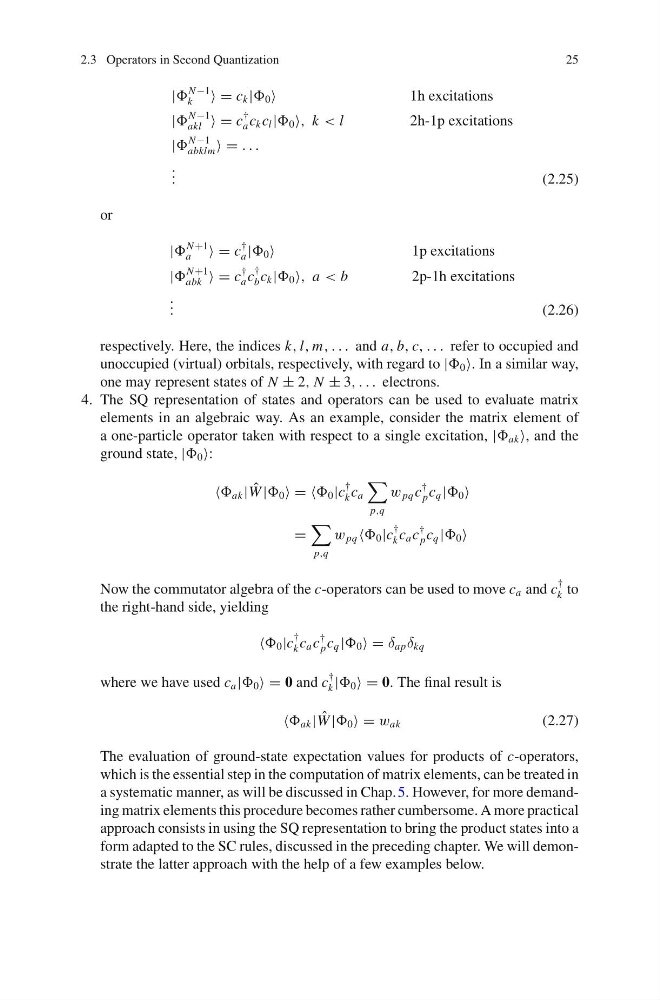
respectively. Here, the indices k, l, m, . . . and a, b, c, . . . refer to occupied and
unoccupied (virtual) orbitals, respectively, with regard to | 0 . In a similar way,
one may represent states of N ± 2, N ± 3, . . . electrons.
4. The SQ representation of states and operators can be used to evaluate matrix
elements in an algebraic way. As an example, consider the matrix element of
a one-particle operator taken with respect to a single excitation, | ak , and the
ground state, | 0 :
ak | ˆ
W | 0 = = 0 |c
†
k c a
p,q
w pq c
†
p c q | 0
=
p,q
w pq 0 |c
†
k c a c
†
p c q | 0
Now the commutator algebra of the c-operators can be used to move c a and c
†
k to
the right-hand side, yielding
0 |c
†
k c a c
†
p c q | 0 = δ ap δ kq
where we have used c a | 0 = 0 and c
†
k | 0 = 0. The final result is
ak | ˆ
W | 0 = w ak
(2.27)
The evaluation of ground-state expectation values for products of c-operators,
which is the essential step in the computation of matrix elements, can be treated in
a systematic manner, as will be discussed in Chap. 5. However, for more demanding matrix elements this procedure becomes rather cumbersome. A more practical
approach consists in using the SQ representation to bring the product states into a
form adapted to the SC rules, discussed in the preceding chapter. We will demonstrate the latter approach with the help of a few examples below.
25
|
N −1
k
= c k | 0
1h excitations
|
N −1
akl = c
†
a c k c l | 0 , k < l
2h-1p excitations
|
N −1
abklm = . . .
. . .
(2.25)
or
|
N +1
a
= c
†
a | 0
1p excitations
|
N +1
abk = c
†
a c
†
b c k | 0 , a < b
2p-1h excitations
. . .
(2.26)
respectively. Here, the indices k, l, m, . . . and a, b, c, . . . refer to occupied and
unoccupied (virtual) orbitals, respectively, with regard to | 0 . In a similar way,
one may represent states of N ± 2, N ± 3, . . . electrons.
4. The SQ representation of states and operators can be used to evaluate matrix
elements in an algebraic way. As an example, consider the matrix element of
a one-particle operator taken with respect to a single excitation, | ak , and the
ground state, | 0 :
ak | ˆ
W | 0 = = 0 |c
†
k c a
p,q
w pq c
†
p c q | 0
=
p,q
w pq 0 |c
†
k c a c
†
p c q | 0
Now the commutator algebra of the c-operators can be used to move c a and c
†
k to
the right-hand side, yielding
0 |c
†
k c a c
†
p c q | 0 = δ ap δ kq
where we have used c a | 0 = 0 and c
†
k | 0 = 0. The final result is
ak | ˆ
W | 0 = w ak
(2.27)
The evaluation of ground-state expectation values for products of c-operators,
which is the essential step in the computation of matrix elements, can be treated in
a systematic manner, as will be discussed in Chap. 5. However, for more demanding matrix elements this procedure becomes rather cumbersome. A more practical
approach consists in using the SQ representation to bring the product states into a
form adapted to the SC rules, discussed in the preceding chapter. We will demonstrate the latter approach with the help of a few examples below.