

26
2 Second Quantization
2.4 Combining Second Quantization and Slater–Condon
Rules
Let us first examine the simple matrix element ak | ˆ
W | 0 . We have found it helpful
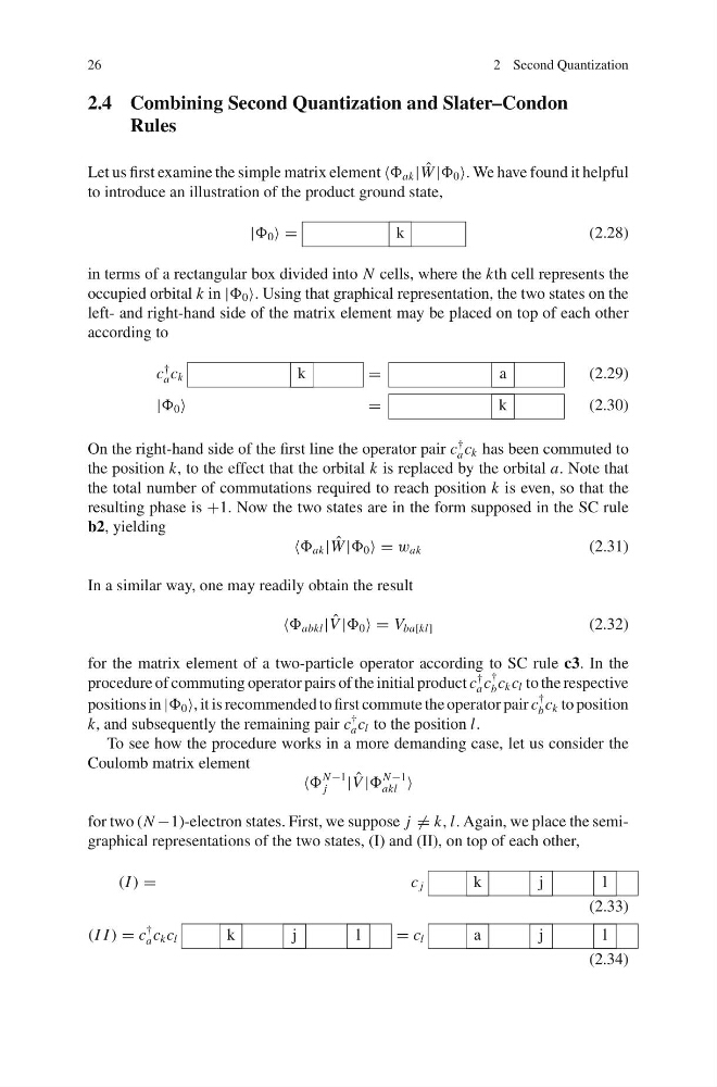
to introduce an illustration of the product ground state,
| 0 =
k
(2.28)
in terms of a rectangular box divided into N cells, where the kth cell represents the
occupied orbital k in | 0 . Using that graphical representation, the two states on the
left- and right-hand side of the matrix element may be placed on top of each other
according to
c
†
a c k
k
=
a
(2.29)
| 0
=
k
(2.30)
On the right-hand side of the first line the operator pair c
†
a c k has been commuted to
the position k, to the effect that the orbital k is replaced by the orbital a. Note that
the total number of commutations required to reach position k is even, so that the
resulting phase is +1. Now the two states are in the form supposed in the SC rule
b2, yielding
ak | ˆ
W | 0 = w ak
(2.31)
In a similar way, one may readily obtain the result
abkl | ˆ
V | 0 = V ba[kl]
(2.32)
for the matrix element of a two-particle operator according to SC rule c3. In the
procedure of commuting operator pairs of the initial product c
†
a c
†
b c k c l to the respective
positions in | 0 , it is recommended to first commute the operator pair c
†
b c k to position
k, and subsequently the remaining pair c
†
a c l to the position l.
To see how the procedure works in a more demanding case, let us consider the
Coulomb matrix element
N −1
j
| ˆ
V |
N −1
akl
for two (N −1)-electron states. First, we suppose j = k, l. Again, we place the semigraphical representations of the two states, (I) and (II), on top of each other,
(I ) =
c j
k
j
l
(2.33)
(I I ) = c
†
a c k c l
k
j
l
= c l
a
j
l
(2.34)
2 Second Quantization
2.4 Combining Second Quantization and Slater–Condon
Rules
Let us first examine the simple matrix element ak | ˆ
W | 0 . We have found it helpful
to introduce an illustration of the product ground state,
| 0 =
k
(2.28)
in terms of a rectangular box divided into N cells, where the kth cell represents the
occupied orbital k in | 0 . Using that graphical representation, the two states on the
left- and right-hand side of the matrix element may be placed on top of each other
according to
c
†
a c k
k
=
a
(2.29)
| 0
=
k
(2.30)
On the right-hand side of the first line the operator pair c
†
a c k has been commuted to
the position k, to the effect that the orbital k is replaced by the orbital a. Note that
the total number of commutations required to reach position k is even, so that the
resulting phase is +1. Now the two states are in the form supposed in the SC rule
b2, yielding
ak | ˆ
W | 0 = w ak
(2.31)
In a similar way, one may readily obtain the result
abkl | ˆ
V | 0 = V ba[kl]
(2.32)
for the matrix element of a two-particle operator according to SC rule c3. In the
procedure of commuting operator pairs of the initial product c
†
a c
†
b c k c l to the respective
positions in | 0 , it is recommended to first commute the operator pair c
†
b c k to position
k, and subsequently the remaining pair c
†
a c l to the position l.
To see how the procedure works in a more demanding case, let us consider the
Coulomb matrix element
N −1
j
| ˆ
V |
N −1
akl
for two (N −1)-electron states. First, we suppose j = k, l. Again, we place the semigraphical representations of the two states, (I) and (II), on top of each other,
(I ) =
c j
k
j
l
(2.33)
(I I ) = c
†
a c k c l
k
j
l
= c l
a
j
l
(2.34)