

Appendix
321
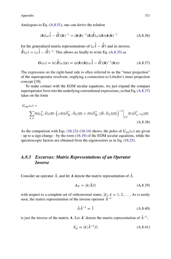
Analogous to Eq. (A.8.51), one can derive the relation
(h|(ω ˆ ˆ
1 − ˆ ˆ
H )|h)
−1
= (h|h)
−1
(h| ˆ ˆ
R(ω)|h)(h|h)
−1
(A.8.36)
for the generalized matrix representations of (ω ˆ ˆ
1 − ˆ ˆ
H ) and its inverse,
ˆ ˆ
R(ω) = (ω ˆ ˆ
1 − ˆ ˆ
H )
−1 . This allows us finally to write Eq. (A.8.35) as
G(ω) = (c| ˆ ˆ
R(ω)|c) = (c|h)(h|(ω ˆ ˆ
1 − ˆ ˆ
H )|h)
−1
(h|c)
(A.8.37)
The expression on the right-hand side is often referred to as the “inner projection”
of the superoperator resolvent, implying a connection to Löwdin’s inner projection
concept [18].
To make contact with the EOM secular equations, we just expand the compact
superoperator form into the underlying conventional expressions, so that Eq. (A.8.37)
takes on the form
G pq (ω) =
I,J
0|{c
†
q , ˆ
O I }|0
ω0|{ ˆ
O
†
K , ˆ
O L }|0 + +0|{ ˆ
O
†
K , [ ˆ
H , ˆ
O L ]}|0
−1
I J
0|{ ˆ
O
†
J , c p }|0
(A.8.38)
As the comparison with Eqs. (16.12)–(16.14) shows, the poles of G pq (ω) are given
- up to a sign change - by the roots (16.19) of the EOM secular equations, while the
spectroscopic factors are obtained from the eigenvectors as in Eq. (16.25).
A.8.3 Excursus: Matrix Representations of an Operator
Inverse
Consider an operator ˆ
A, and let A denote the matrix representation of ˆ
A,
A kl = =k| ˆ
A|l
(A.8.39)
with respect to a complete set of orthonormal states, |k, k = 1, 2, . . . . As is easily
seen, the matrix representation of the inverse operator ˆ
A
−1
ˆ
A ˆ
A
−1
= ˆ
1
(A.8.40)
is just the inverse of the matrix A. Let A
denote the matrix representation of ˆ
A
−1 ,
A
kl = =k| ˆ
A
−1
|l
(A.8.41)
321
Analogous to Eq. (A.8.51), one can derive the relation
(h|(ω ˆ ˆ
1 − ˆ ˆ
H )|h)
−1
= (h|h)
−1
(h| ˆ ˆ
R(ω)|h)(h|h)
−1
(A.8.36)
for the generalized matrix representations of (ω ˆ ˆ
1 − ˆ ˆ
H ) and its inverse,
ˆ ˆ
R(ω) = (ω ˆ ˆ
1 − ˆ ˆ
H )
−1 . This allows us finally to write Eq. (A.8.35) as
G(ω) = (c| ˆ ˆ
R(ω)|c) = (c|h)(h|(ω ˆ ˆ
1 − ˆ ˆ
H )|h)
−1
(h|c)
(A.8.37)
The expression on the right-hand side is often referred to as the “inner projection”
of the superoperator resolvent, implying a connection to Löwdin’s inner projection
concept [18].
To make contact with the EOM secular equations, we just expand the compact
superoperator form into the underlying conventional expressions, so that Eq. (A.8.37)
takes on the form
G pq (ω) =
I,J
0|{c
†
q , ˆ
O I }|0
ω0|{ ˆ
O
†
K , ˆ
O L }|0 + +0|{ ˆ
O
†
K , [ ˆ
H , ˆ
O L ]}|0
−1
I J
0|{ ˆ
O
†
J , c p }|0
(A.8.38)
As the comparison with Eqs. (16.12)–(16.14) shows, the poles of G pq (ω) are given
- up to a sign change - by the roots (16.19) of the EOM secular equations, while the
spectroscopic factors are obtained from the eigenvectors as in Eq. (16.25).
A.8.3 Excursus: Matrix Representations of an Operator
Inverse
Consider an operator ˆ
A, and let A denote the matrix representation of ˆ
A,
A kl = =k| ˆ
A|l
(A.8.39)
with respect to a complete set of orthonormal states, |k, k = 1, 2, . . . . As is easily
seen, the matrix representation of the inverse operator ˆ
A
−1
ˆ
A ˆ
A
−1
= ˆ
1
(A.8.40)
is just the inverse of the matrix A. Let A
denote the matrix representation of ˆ
A
−1 ,
A
kl = =k| ˆ
A
−1
|l
(A.8.41)