

Appendix
315
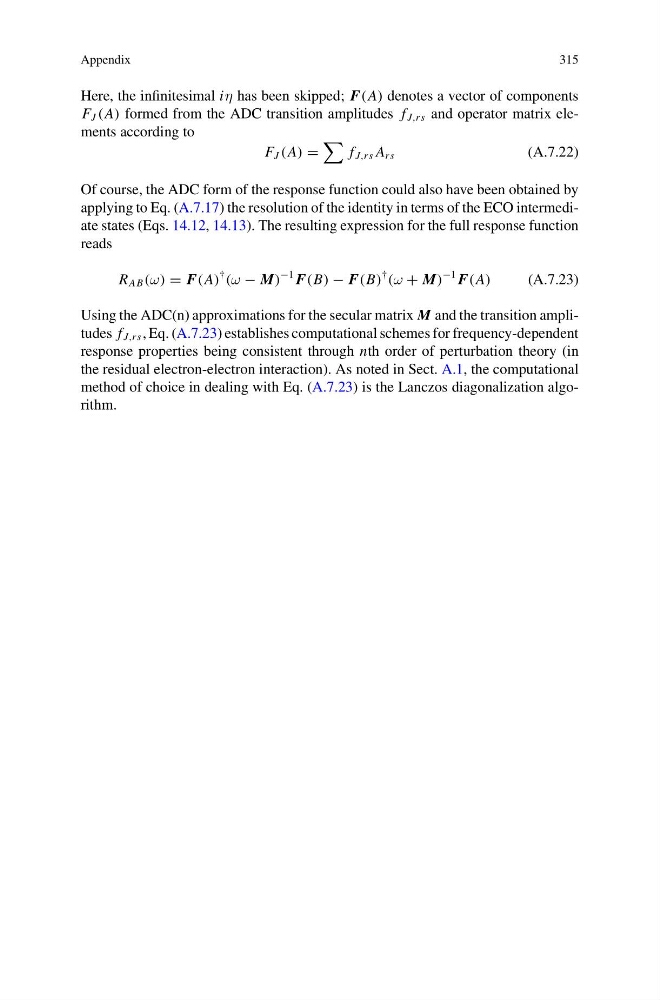
Here, the infinitesimal iη has been skipped; F(A) denotes a vector of components
F J (A) formed from the ADC transition amplitudes f J,rs and operator matrix elements according to
F J (A) =
f J,rs A rs
(A.7.22)
Of course, the ADC form of the response function could also have been obtained by
applying to Eq. (A.7.17) the resolution of the identity in terms of the ECO intermediate states (Eqs. 14.12, 14.13). The resulting expression for the full response function
reads
R AB (ω) = F(A)
†
(ω − M)
−1 F(B) − F(B)
†
(ω + M)
−1 F(A)
(A.7.23)
Using the ADC(n) approximations for the secular matrix M and the transition amplitudes f J,rs , Eq. (A.7.23) establishes computational schemes for frequency-dependent
response properties being consistent through nth order of perturbation theory (in
the residual electron-electron interaction). As noted in Sect. A.1, the computational
method of choice in dealing with Eq. (A.7.23) is the Lanczos diagonalization algorithm.
315
Here, the infinitesimal iη has been skipped; F(A) denotes a vector of components
F J (A) formed from the ADC transition amplitudes f J,rs and operator matrix elements according to
F J (A) =
f J,rs A rs
(A.7.22)
Of course, the ADC form of the response function could also have been obtained by
applying to Eq. (A.7.17) the resolution of the identity in terms of the ECO intermediate states (Eqs. 14.12, 14.13). The resulting expression for the full response function
reads
R AB (ω) = F(A)
†
(ω − M)
−1 F(B) − F(B)
†
(ω + M)
−1 F(A)
(A.7.23)
Using the ADC(n) approximations for the secular matrix M and the transition amplitudes f J,rs , Eq. (A.7.23) establishes computational schemes for frequency-dependent
response properties being consistent through nth order of perturbation theory (in
the residual electron-electron interaction). As noted in Sect. A.1, the computational
method of choice in dealing with Eq. (A.7.23) is the Lanczos diagonalization algorithm.