

302
Appendix
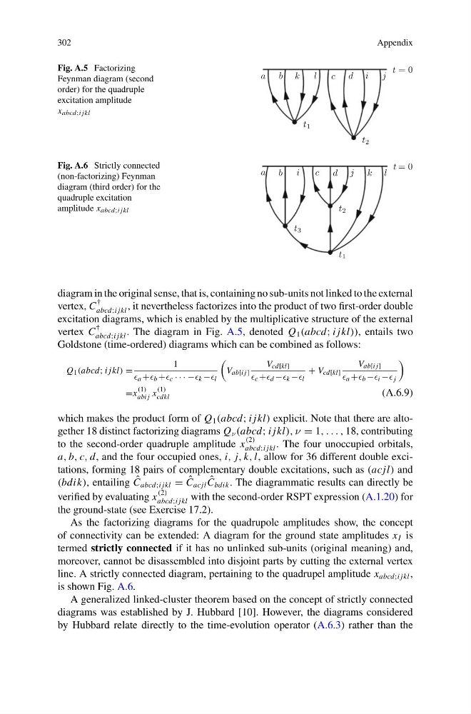
Fig. A.5 Factorizing
Feynman diagram (second
order) for the quadruple
excitation amplitude
x abcd;i jkl
a b k
l
t = 0
c d i j
t 1
t 2
Fig. A.6 Strictly connected
(non-factorizing) Feynman
diagram (third order) for the
quadruple excitation
amplitude x abcd;i jkl
a b
i
c
t = 0
d j k l
t 3
t 2
t 1
diagram in the original sense, that is, containing no sub-units not linked to the external
vertex, C
†
abcd;i jkl , it nevertheless factorizes into the product of two first-order double
excitation diagrams, which is enabled by the multiplicative structure of the external
vertex C
†
abcd;i jkl . The diagram in Fig. A.5, denoted Q 1 (abcd; i jkl)), entails two
Goldstone (time-ordered) diagrams which can be combined as follows:
Q 1 (abcd; i jkl) =
1
a + b + c · · · − k − l
V ab[i j]
V cd[kl]
c + d − k − l
+ V cd[kl]
V ab[i j]
a + b − i − j
=x
(1)
abi j x
(1)
cdkl
(A.6.9)
which makes the product form of Q 1 (abcd; i jkl) explicit. Note that there are altogether 18 distinct factorizing diagrams Q ν (abcd; i jkl), ν = 1, . . . , 18, contributing
to the second-order quadruple amplitude x
(2)
abcd;i jkl . The four unoccupied orbitals,
a, b, c, d, and the four occupied ones, i, j, k, l, allow for 36 different double excitations, forming 18 pairs of complementary double excitations, such as (acjl) and
(bdik), entailing ˆ
C abcd;i jkl = ˆ
C acjl ˆ
C bdik . The diagrammatic results can directly be
verified by evaluating x
(2)
abcd;i jkl with the second-order RSPT expression (A.1.20) for
the ground-state (see Exercise 17.2).
As the factorizing diagrams for the quadrupole amplitudes show, the concept
of connectivity can be extended: A diagram for the ground state amplitudes x I is
termed strictly connected if it has no unlinked sub-units (original meaning) and,
moreover, cannot be disassembled into disjoint parts by cutting the external vertex
line. A strictly connected diagram, pertaining to the quadrupel amplitude x abcd;i jkl ,
is shown Fig. A.6.
A generalized linked-cluster theorem based on the concept of strictly connected
diagrams was established by J. Hubbard [10]. However, the diagrams considered
by Hubbard relate directly to the time-evolution operator (A.6.3) rather than the
Appendix
Fig. A.5 Factorizing
Feynman diagram (second
order) for the quadruple
excitation amplitude
x abcd;i jkl
a b k
l
t = 0
c d i j
t 1
t 2
Fig. A.6 Strictly connected
(non-factorizing) Feynman
diagram (third order) for the
quadruple excitation
amplitude x abcd;i jkl
a b
i
c
t = 0
d j k l
t 3
t 2
t 1
diagram in the original sense, that is, containing no sub-units not linked to the external
vertex, C
†
abcd;i jkl , it nevertheless factorizes into the product of two first-order double
excitation diagrams, which is enabled by the multiplicative structure of the external
vertex C
†
abcd;i jkl . The diagram in Fig. A.5, denoted Q 1 (abcd; i jkl)), entails two
Goldstone (time-ordered) diagrams which can be combined as follows:
Q 1 (abcd; i jkl) =
1
a + b + c · · · − k − l
V ab[i j]
V cd[kl]
c + d − k − l
+ V cd[kl]
V ab[i j]
a + b − i − j
=x
(1)
abi j x
(1)
cdkl
(A.6.9)
which makes the product form of Q 1 (abcd; i jkl) explicit. Note that there are altogether 18 distinct factorizing diagrams Q ν (abcd; i jkl), ν = 1, . . . , 18, contributing
to the second-order quadruple amplitude x
(2)
abcd;i jkl . The four unoccupied orbitals,
a, b, c, d, and the four occupied ones, i, j, k, l, allow for 36 different double excitations, forming 18 pairs of complementary double excitations, such as (acjl) and
(bdik), entailing ˆ
C abcd;i jkl = ˆ
C acjl ˆ
C bdik . The diagrammatic results can directly be
verified by evaluating x
(2)
abcd;i jkl with the second-order RSPT expression (A.1.20) for
the ground-state (see Exercise 17.2).
As the factorizing diagrams for the quadrupole amplitudes show, the concept
of connectivity can be extended: A diagram for the ground state amplitudes x I is
termed strictly connected if it has no unlinked sub-units (original meaning) and,
moreover, cannot be disassembled into disjoint parts by cutting the external vertex
line. A strictly connected diagram, pertaining to the quadrupel amplitude x abcd;i jkl ,
is shown Fig. A.6.
A generalized linked-cluster theorem based on the concept of strictly connected
diagrams was established by J. Hubbard [10]. However, the diagrams considered
by Hubbard relate directly to the time-evolution operator (A.6.3) rather than the