

Appendix
301
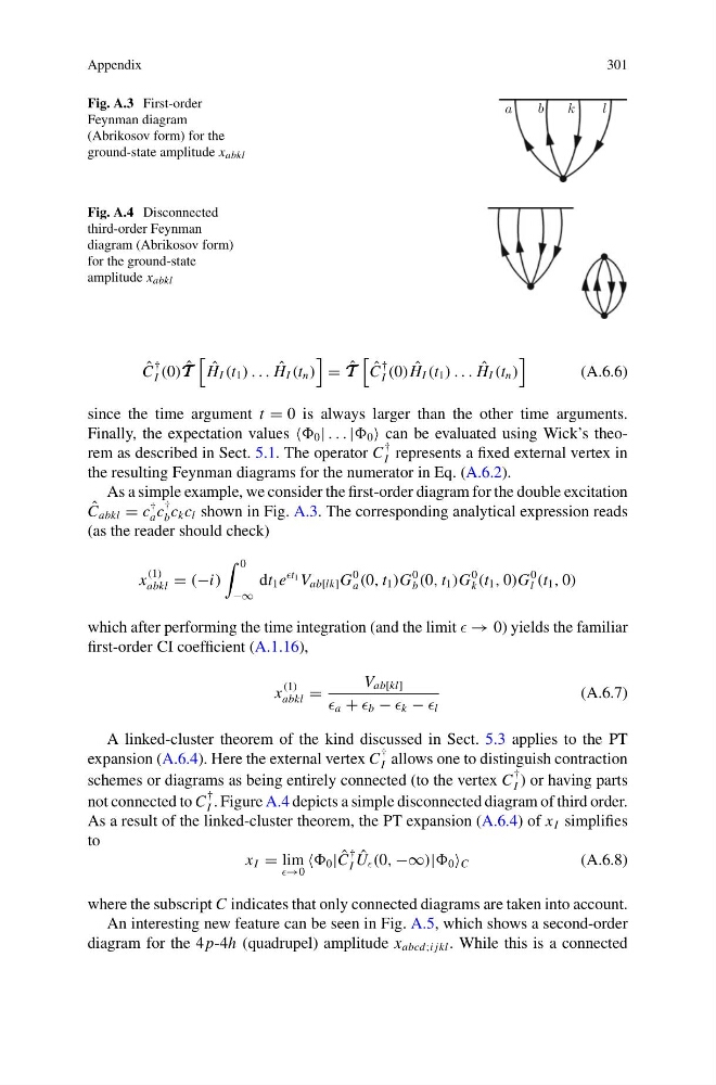
Fig. A.3 First-order
Feynman diagram
(Abrikosov form) for the
ground-state amplitude x abkl
a
b
k
l
Fig. A.4 Disconnected
third-order Feynman
diagram (Abrikosov form)
for the ground-state
amplitude x abkl
ˆ
C
†
I (0) ˆ
T T T
ˆ
H I (t 1 ) . . . ˆ
H I (t n )
= ˆ
T T T
ˆ
C
†
I (0) ˆ
H I (t 1 ) . . . ˆ
H I (t n )
(A.6.6)
since the time argument t = 0 is always larger than the other time arguments.
Finally, the expectation values 0 | . . . | 0 can be evaluated using Wick’s theorem as described in Sect. 5.1. The operator C
†
I represents a fixed external vertex in
the resulting Feynman diagrams for the numerator in Eq. (A.6.2).
As a simple example, we consider the first-order diagram for the double excitation
ˆ
C abkl = c
†
a c
†
b c k c l shown in Fig. A.3. The corresponding analytical expression reads
(as the reader should check)
x
(1)
abkl = (−i)
0
−∞
dt 1 e
t 1 V ab[lk] G
0
a (0, t 1 )G
0
b (0, t 1 )G
0
k (t 1 , 0)G
0
l (t 1 , 0)
which after performing the time integration (and the limit → 0) yields the familiar
first-order CI coefficient (A.1.16),
x
(1)
abkl =
V ab[kl]
a + b − k − l
(A.6.7)
A linked-cluster theorem of the kind discussed in Sect. 5.3 applies to the PT
expansion (A.6.4). Here the external vertex C
†
I allows one to distinguish contraction
schemes or diagrams as being entirely connected (to the vertex C
†
I ) or having parts
not connected to C
†
I . Figure A.4 depicts a simple disconnected diagram of third order.
As a result of the linked-cluster theorem, the PT expansion (A.6.4) of x I simplifies
to
x I = lim
→0
0 | ˆ
C
†
I
ˆ
U (0, −∞)| 0 C
(A.6.8)
where the subscript C indicates that only connected diagrams are taken into account.
An interesting new feature can be seen in Fig. A.5, which shows a second-order
diagram for the 4 p-4h (quadrupel) amplitude x abcd;i jkl . While this is a connected
301
Fig. A.3 First-order
Feynman diagram
(Abrikosov form) for the
ground-state amplitude x abkl
a
b
k
l
Fig. A.4 Disconnected
third-order Feynman
diagram (Abrikosov form)
for the ground-state
amplitude x abkl
ˆ
C
†
I (0) ˆ
T T T
ˆ
H I (t 1 ) . . . ˆ
H I (t n )
= ˆ
T T T
ˆ
C
†
I (0) ˆ
H I (t 1 ) . . . ˆ
H I (t n )
(A.6.6)
since the time argument t = 0 is always larger than the other time arguments.
Finally, the expectation values 0 | . . . | 0 can be evaluated using Wick’s theorem as described in Sect. 5.1. The operator C
†
I represents a fixed external vertex in
the resulting Feynman diagrams for the numerator in Eq. (A.6.2).
As a simple example, we consider the first-order diagram for the double excitation
ˆ
C abkl = c
†
a c
†
b c k c l shown in Fig. A.3. The corresponding analytical expression reads
(as the reader should check)
x
(1)
abkl = (−i)
0
−∞
dt 1 e
t 1 V ab[lk] G
0
a (0, t 1 )G
0
b (0, t 1 )G
0
k (t 1 , 0)G
0
l (t 1 , 0)
which after performing the time integration (and the limit → 0) yields the familiar
first-order CI coefficient (A.1.16),
x
(1)
abkl =
V ab[kl]
a + b − k − l
(A.6.7)
A linked-cluster theorem of the kind discussed in Sect. 5.3 applies to the PT
expansion (A.6.4). Here the external vertex C
†
I allows one to distinguish contraction
schemes or diagrams as being entirely connected (to the vertex C
†
I ) or having parts
not connected to C
†
I . Figure A.4 depicts a simple disconnected diagram of third order.
As a result of the linked-cluster theorem, the PT expansion (A.6.4) of x I simplifies
to
x I = lim
→0
0 | ˆ
C
†
I
ˆ
U (0, −∞)| 0 C
(A.6.8)
where the subscript C indicates that only connected diagrams are taken into account.
An interesting new feature can be seen in Fig. A.5, which shows a second-order
diagram for the 4 p-4h (quadrupel) amplitude x abcd;i jkl . While this is a connected