

Appendix
303
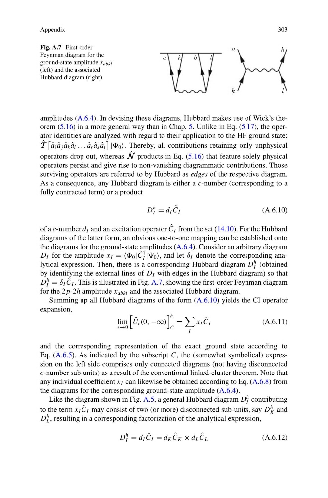
Fig. A.7 First-order
Feynman diagram for the
ground-state amplitude x abkl
(left) and the associated
Hubbard diagram (right)
a
k
b
l
a
b
k
l
amplitudes (A.6.4). In devising these diagrams, Hubbard makes use of Wick’s theorem (5.16) in a more general way than in Chap. 5. Unlike in Eq. (5.17), the operator identities are analyzed with regard to their application to the HF ground state:
ˆ
T T T
ˆ
a i ˆ
a j ˆ
a k ˆ
a l . . . ˆ
a r ˆ
a s ˆ
a t
| 0 . Thereby, all contributions retaining only unphysical
operators drop out, whereas ˆ
N N N products in Eq. (5.16) that feature solely physical
operators persist and give rise to non-vanishing diagrammatic contributions. Those
surviving operators are referred to by Hubbard as edges of the respective diagram.
As a consequence, any Hubbard diagram is either a c-number (corresponding to a
fully contracted term) or a product
D
h
I = d I ˆ
C I
(A.6.10)
of a c-number d I and an excitation operator ˆ
C I from the set (14.10). For the Hubbard
diagrams of the latter form, an obvious one-to-one mapping can be established onto
the diagrams for the ground-state amplitudes (A.6.4). Consider an arbitrary diagram
D I for the amplitude x I = = 0 | ˆ
C
†
I | 0 , and let δ I denote the corresponding analytical expression. Then, there is a corresponding Hubbard diagram D
h
I (obtained
by identifying the external lines of D I with edges in the Hubbard diagram) so that
D
h
I = δ I ˆ
C I . This is illustrated in Fig. A.7, showing the first-order Feynman diagram
for the 2 p-2h amplitude x abkl and the associated Hubbard diagram.
Summing up all Hubbard diagrams of the form (A.6.10) yields the CI operator
expansion,
lim
→0
ˆ
U (0, −∞)
h
C
=
I
x I ˆ
C I
(A.6.11)
and the corresponding representation of the exact ground state according to
Eq. (A.6.5). As indicated by the subscript C, the (somewhat symbolical) expression on the left side comprises only connected diagrams (not having disconnected
c-number sub-units) as a result of the conventional linked-cluster theorem. Note that
any individual coefficient x I can likewise be obtained according to Eq. (A.6.8) from
the diagrams for the corresponding ground-state amplitude (A.6.4).
Like the diagram shown in Fig. A.5, a general Hubbard diagram D
h
I contributing
to the term x I ˆ
C I may consist of two (or more) disconnected sub-units, say D
h
K and
D
h
L , resulting in a corresponding factorization of the analytical expression,
D
h
I = d I ˆ
C I = d K ˆ
C K × d L ˆ
C L
(A.6.12)
303
Fig. A.7 First-order
Feynman diagram for the
ground-state amplitude x abkl
(left) and the associated
Hubbard diagram (right)
a
k
b
l
a
b
k
l
amplitudes (A.6.4). In devising these diagrams, Hubbard makes use of Wick’s theorem (5.16) in a more general way than in Chap. 5. Unlike in Eq. (5.17), the operator identities are analyzed with regard to their application to the HF ground state:
ˆ
T T T
ˆ
a i ˆ
a j ˆ
a k ˆ
a l . . . ˆ
a r ˆ
a s ˆ
a t
| 0 . Thereby, all contributions retaining only unphysical
operators drop out, whereas ˆ
N N N products in Eq. (5.16) that feature solely physical
operators persist and give rise to non-vanishing diagrammatic contributions. Those
surviving operators are referred to by Hubbard as edges of the respective diagram.
As a consequence, any Hubbard diagram is either a c-number (corresponding to a
fully contracted term) or a product
D
h
I = d I ˆ
C I
(A.6.10)
of a c-number d I and an excitation operator ˆ
C I from the set (14.10). For the Hubbard
diagrams of the latter form, an obvious one-to-one mapping can be established onto
the diagrams for the ground-state amplitudes (A.6.4). Consider an arbitrary diagram
D I for the amplitude x I = = 0 | ˆ
C
†
I | 0 , and let δ I denote the corresponding analytical expression. Then, there is a corresponding Hubbard diagram D
h
I (obtained
by identifying the external lines of D I with edges in the Hubbard diagram) so that
D
h
I = δ I ˆ
C I . This is illustrated in Fig. A.7, showing the first-order Feynman diagram
for the 2 p-2h amplitude x abkl and the associated Hubbard diagram.
Summing up all Hubbard diagrams of the form (A.6.10) yields the CI operator
expansion,
lim
→0
ˆ
U (0, −∞)
h
C
=
I
x I ˆ
C I
(A.6.11)
and the corresponding representation of the exact ground state according to
Eq. (A.6.5). As indicated by the subscript C, the (somewhat symbolical) expression on the left side comprises only connected diagrams (not having disconnected
c-number sub-units) as a result of the conventional linked-cluster theorem. Note that
any individual coefficient x I can likewise be obtained according to Eq. (A.6.8) from
the diagrams for the corresponding ground-state amplitude (A.6.4).
Like the diagram shown in Fig. A.5, a general Hubbard diagram D
h
I contributing
to the term x I ˆ
C I may consist of two (or more) disconnected sub-units, say D
h
K and
D
h
L , resulting in a corresponding factorization of the analytical expression,
D
h
I = d I ˆ
C I = d K ˆ
C K × d L ˆ
C L
(A.6.12)