

298
Appendix
in Chap. 9, the explicit computation of the self-energy pole positions and residue
amplitudes can be circumvented as described in the following.
According to Eq. (9.2), each of the M
±
(ω) parts can be written in the ADC form
M
±
pq (ω) = (U
±
p )
†
ω − K
±
− C
±
−1 U
±
q
(A.5.20)
where K
±
+ C
± and U
±
p are the secular matrices and coupling vectors as given at
the respective ADC level. The associated ADC eigenvalue equations (9.27)
(K
±
+ C
±
)Y
±
= Y
±
±
, (Y
±
)
† Y
±
= 1
(A.5.21)
determine the pole positions as the eigenvalues ω n , and the residue amplitudes (9.28)
according to
m np = (Y
±
n )
† U
±
p
(A.5.22)
In view of the size of the ADC secular matrices, their full diagonalization, needed to
obtain all eigenvalues and residue amplitudes, is obviously not a viable computational
strategy. For an alternative approach, we introduce the (column) vectors
V
+
k = ( k 1 − K
+
− C
+
)
−1 U
+
k
(A.5.23)
for occupied orbitals, k, and
V
−
a = ( a 1 − K
−
− C
−
)
−1 U
−
a
(A.5.24)
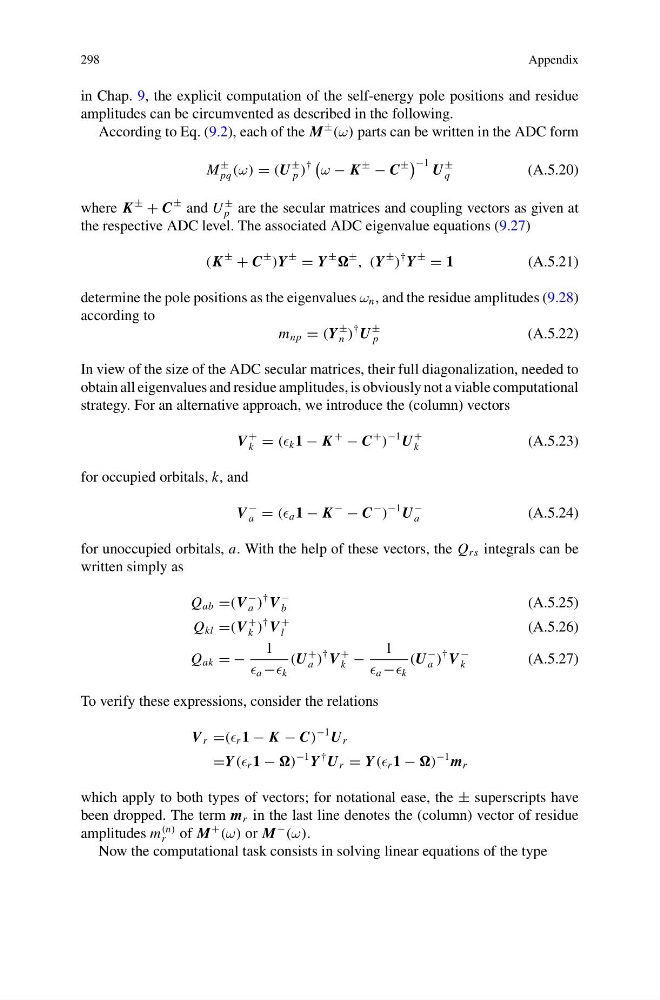
for unoccupied orbitals, a. With the help of these vectors, the Q rs integrals can be
written simply as
Q ab =(V
−
a )
† V
−
b
(A.5.25)
Q kl =(V
+
k )
† V
+
l
(A.5.26)
Q ak = −
1
a − k
(U
+
a )
† V
+
k −
1
a − k
(U
−
a )
† V
−
k
(A.5.27)
To verify these expressions, consider the relations
V r =( r 1 − K − C)
−1 U r
=Y ( r 1 − )
−1 Y
† U r = Y ( r 1 − )
−1 m r
which apply to both types of vectors; for notational ease, the ± superscripts have
been dropped. The term m r in the last line denotes the (column) vector of residue
amplitudes m
(n)
r of M
+
(ω) or M
−
(ω).
Now the computational task consists in solving linear equations of the type
Appendix
in Chap. 9, the explicit computation of the self-energy pole positions and residue
amplitudes can be circumvented as described in the following.
According to Eq. (9.2), each of the M
±
(ω) parts can be written in the ADC form
M
±
pq (ω) = (U
±
p )
†
ω − K
±
− C
±
−1 U
±
q
(A.5.20)
where K
±
+ C
± and U
±
p are the secular matrices and coupling vectors as given at
the respective ADC level. The associated ADC eigenvalue equations (9.27)
(K
±
+ C
±
)Y
±
= Y
±
±
, (Y
±
)
† Y
±
= 1
(A.5.21)
determine the pole positions as the eigenvalues ω n , and the residue amplitudes (9.28)
according to
m np = (Y
±
n )
† U
±
p
(A.5.22)
In view of the size of the ADC secular matrices, their full diagonalization, needed to
obtain all eigenvalues and residue amplitudes, is obviously not a viable computational
strategy. For an alternative approach, we introduce the (column) vectors
V
+
k = ( k 1 − K
+
− C
+
)
−1 U
+
k
(A.5.23)
for occupied orbitals, k, and
V
−
a = ( a 1 − K
−
− C
−
)
−1 U
−
a
(A.5.24)
for unoccupied orbitals, a. With the help of these vectors, the Q rs integrals can be
written simply as
Q ab =(V
−
a )
† V
−
b
(A.5.25)
Q kl =(V
+
k )
† V
+
l
(A.5.26)
Q ak = −
1
a − k
(U
+
a )
† V
+
k −
1
a − k
(U
−
a )
† V
−
k
(A.5.27)
To verify these expressions, consider the relations
V r =( r 1 − K − C)
−1 U r
=Y ( r 1 − )
−1 Y
† U r = Y ( r 1 − )
−1 m r
which apply to both types of vectors; for notational ease, the ± superscripts have
been dropped. The term m r in the last line denotes the (column) vector of residue
amplitudes m
(n)
r of M
+
(ω) or M
−
(ω).
Now the computational task consists in solving linear equations of the type