

Appendix
297
Thus, the formal solution of the linear set of equations takes on the form
ph
(∞) = (1 − A
ph
)
−1 b
ph
(A.5.13)
Once the p-h and h- p components of (∞) have been obtained by solving the
Eqs. (A.5.9) or (A.5.10), the h-h and p- p matrix elements can be evaluated according
to
i j (∞) =
b,l
1
l − b
(V il[ jb] bl (∞) + V ib[ jl] lb (∞)) + b i j
(A.5.14)
ac (∞) =
b,l
1
l − b
(V al[cb] bl (∞) + V ab[cl] lb (∞)) + b ac
(A.5.15)
Treatment of the Inhomogenities
The inhomogenities b pq , as given by Eqs. (A.5.6), (A.5.7), establish the connection
with the dynamic part M(ω) of the self-energy via the contour integrals (A.5.7). If
M(ω) is available in the explicit form of spectral representation (8.19), the contour
integrals Q rs can readily be evaluated. Here, it is useful to distinguish between p- p,
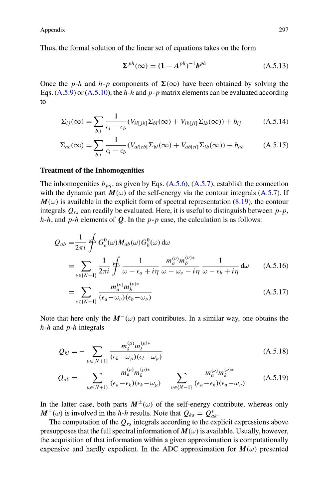
h-h, and p-h elements of Q. In the p- p case, the calculation is as follows:
Q ab =
1
2πi
2 G
0
a (ω)M ab (ω)G
0
b (ω) dω
=
ν∈{N −1}
1
2πi
2
1
ω − a + iη
m
(ν)
a m
(ν)∗
b
ω − ω ν − iη
1
ω − b + iη
dω
(A.5.16)
=
ν∈{N −1}
m
(ν)
a m
(ν)∗
b
( a −ω ν )( b −ω ν )
(A.5.17)
Note that here only the M
−
(ω) part contributes. In a similar way, one obtains the
h-h and p-h integrals
Q kl = −
μ∈{N +1}
m
(μ)
k m
(μ)∗
l
( k −ω μ )( l −ω μ )
(A.5.18)
Q ak = −
μ∈{N +1}
m
(μ)
a m
(μ)∗
k
( a − k )( k −ω μ )
−
ν∈{N −1}
m
(ν)
a m
(ν)∗
k
( a − k )( a −ω ν )
(A.5.19)
In the latter case, both parts M
±
(ω) of the self-energy contribute, whereas only
M
+
(ω) is involved in the h-h results. Note that Q ka = Q
∗
ak .
The computation of the Q rs integrals according to the explicit expressions above
presupposes that the full spectral information of M(ω) is available. Usually, however,
the acquisition of that information within a given approximation is computationally
expensive and hardly expedient. In the ADC approximation for M(ω) presented
297
Thus, the formal solution of the linear set of equations takes on the form
ph
(∞) = (1 − A
ph
)
−1 b
ph
(A.5.13)
Once the p-h and h- p components of (∞) have been obtained by solving the
Eqs. (A.5.9) or (A.5.10), the h-h and p- p matrix elements can be evaluated according
to
i j (∞) =
b,l
1
l − b
(V il[ jb] bl (∞) + V ib[ jl] lb (∞)) + b i j
(A.5.14)
ac (∞) =
b,l
1
l − b
(V al[cb] bl (∞) + V ab[cl] lb (∞)) + b ac
(A.5.15)
Treatment of the Inhomogenities
The inhomogenities b pq , as given by Eqs. (A.5.6), (A.5.7), establish the connection
with the dynamic part M(ω) of the self-energy via the contour integrals (A.5.7). If
M(ω) is available in the explicit form of spectral representation (8.19), the contour
integrals Q rs can readily be evaluated. Here, it is useful to distinguish between p- p,
h-h, and p-h elements of Q. In the p- p case, the calculation is as follows:
Q ab =
1
2πi
2 G
0
a (ω)M ab (ω)G
0
b (ω) dω
=
ν∈{N −1}
1
2πi
2
1
ω − a + iη
m
(ν)
a m
(ν)∗
b
ω − ω ν − iη
1
ω − b + iη
dω
(A.5.16)
=
ν∈{N −1}
m
(ν)
a m
(ν)∗
b
( a −ω ν )( b −ω ν )
(A.5.17)
Note that here only the M
−
(ω) part contributes. In a similar way, one obtains the
h-h and p-h integrals
Q kl = −
μ∈{N +1}
m
(μ)
k m
(μ)∗
l
( k −ω μ )( l −ω μ )
(A.5.18)
Q ak = −
μ∈{N +1}
m
(μ)
a m
(μ)∗
k
( a − k )( k −ω μ )
−
ν∈{N −1}
m
(ν)
a m
(ν)∗
k
( a − k )( a −ω ν )
(A.5.19)
In the latter case, both parts M
±
(ω) of the self-energy contribute, whereas only
M
+
(ω) is involved in the h-h results. Note that Q ka = Q
∗
ak .
The computation of the Q rs integrals according to the explicit expressions above
presupposes that the full spectral information of M(ω) is available. Usually, however,
the acquisition of that information within a given approximation is computationally
expensive and hardly expedient. In the ADC approximation for M(ω) presented