

296
Appendix
where O(5) indicates that the truncation error for pq (∞) is of fifth order. The
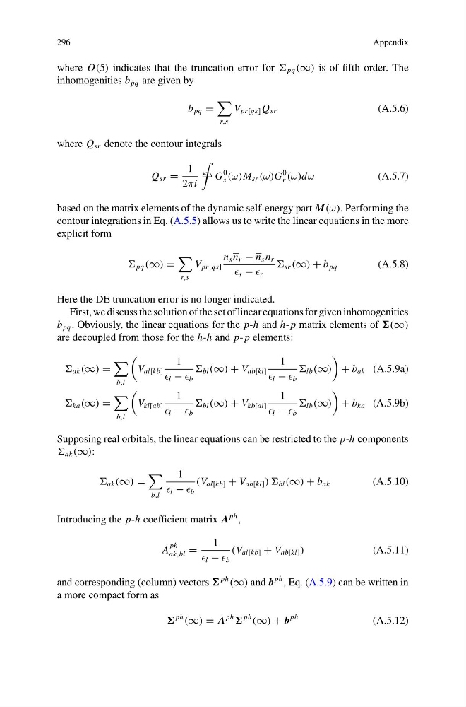
inhomogenities b pq are given by
b pq =
r,s
V pr[qs] Q sr
(A.5.6)
where Q sr denote the contour integrals
Q sr =
1
2πi
2 G
0
s (ω)M sr (ω)G
0
r (ω)dω
(A.5.7)
based on the matrix elements of the dynamic self-energy part M(ω). Performing the
contour integrations in Eq. (A.5.5) allows us to write the linear equations in the more
explicit form
pq (∞) =
r,s
V pr[qs]
n s n r − n s n r
s − r
sr (∞) + b pq
(A.5.8)
Here the DE truncation error is no longer indicated.
First, we discuss the solution of the set of linear equations for given inhomogenities
b pq . Obviously, the linear equations for the p-h and h- p matrix elements of (∞)
are decoupled from those for the h-h and p- p elements:
ak (∞) =
b,l
V al[kb]
1
l − b
bl (∞) + V ab[kl]
1
l − b
lb (∞)
+ b ak (A.5.9a)
ka (∞) =
b,l
V kl[ab]
1
l − b
bl (∞) + V kb[al]
1
l − b
lb (∞)
+ b ka (A.5.9b)
Supposing real orbitals, the linear equations can be restricted to the p-h components
ak (∞):
ak (∞) =
b,l
1
l − b
(V al[kb] + V ab[kl] ) ) bl (∞) + b ak
(A.5.10)
Introducing the p-h coefficient matrix A
ph ,
A
ph
ak,bl =
1
l − b
(V al[kb] + V ab[kl] )
(A.5.11)
and corresponding (column) vectors
ph
(∞) and b
ph , Eq. (A.5.9) can be written in
a more compact form as
ph
(∞) = A
ph
ph
(∞) + b
ph
(A.5.12)
Appendix
where O(5) indicates that the truncation error for pq (∞) is of fifth order. The
inhomogenities b pq are given by
b pq =
r,s
V pr[qs] Q sr
(A.5.6)
where Q sr denote the contour integrals
Q sr =
1
2πi
2 G
0
s (ω)M sr (ω)G
0
r (ω)dω
(A.5.7)
based on the matrix elements of the dynamic self-energy part M(ω). Performing the
contour integrations in Eq. (A.5.5) allows us to write the linear equations in the more
explicit form
pq (∞) =
r,s
V pr[qs]
n s n r − n s n r
s − r
sr (∞) + b pq
(A.5.8)
Here the DE truncation error is no longer indicated.
First, we discuss the solution of the set of linear equations for given inhomogenities
b pq . Obviously, the linear equations for the p-h and h- p matrix elements of (∞)
are decoupled from those for the h-h and p- p elements:
ak (∞) =
b,l
V al[kb]
1
l − b
bl (∞) + V ab[kl]
1
l − b
lb (∞)
+ b ak (A.5.9a)
ka (∞) =
b,l
V kl[ab]
1
l − b
bl (∞) + V kb[al]
1
l − b
lb (∞)
+ b ka (A.5.9b)
Supposing real orbitals, the linear equations can be restricted to the p-h components
ak (∞):
ak (∞) =
b,l
1
l − b
(V al[kb] + V ab[kl] ) ) bl (∞) + b ak
(A.5.10)
Introducing the p-h coefficient matrix A
ph ,
A
ph
ak,bl =
1
l − b
(V al[kb] + V ab[kl] )
(A.5.11)
and corresponding (column) vectors
ph
(∞) and b
ph , Eq. (A.5.9) can be written in
a more compact form as
ph
(∞) = A
ph
ph
(∞) + b
ph
(A.5.12)