

Appendix
289
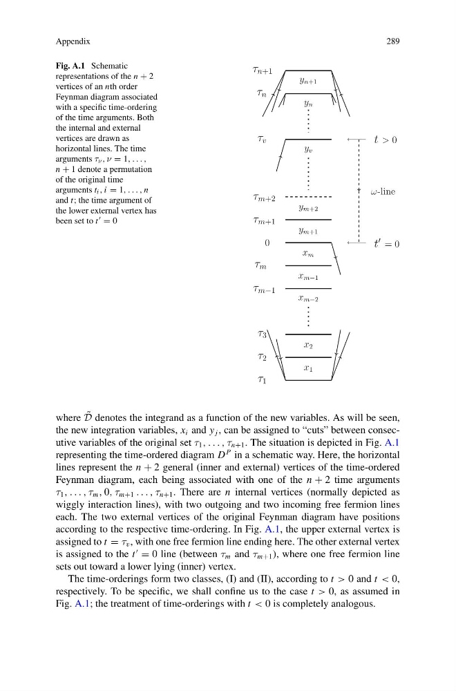
Fig. A.1 Schematic
representations of the n + 2
vertices of an nth order
Feynman diagram associated
with a specific time-ordering
of the time arguments. Both
the internal and external
vertices are drawn as
horizontal lines. The time
arguments τ ν , ν = 1, . . . ,
n + 1 denote a permutation
of the original time
arguments t i , i = 1, . . . , n
and t; the time argument of
the lower external vertex has
been set to t = 0
τ n+1
y n+1
τ n
y n
τ v
y v
t > 0
ω-line
τ m+2
y m+2
τ m+1
y m+1
0
x m
t
= 0
τ m
x m−1
τ m−1
x m−2
τ 3
x 2
τ 2
x 1
τ 1
where ˜
D denotes the integrand as a function of the new variables. As will be seen,
the new integration variables, x i and y j , can be assigned to “cuts” between consecutive variables of the original set τ 1 , . . . , τ n+1 . The situation is depicted in Fig. A.1
representing the time-ordered diagram D
P in a schematic way. Here, the horizontal
lines represent the n + 2 general (inner and external) vertices of the time-ordered
Feynman diagram, each being associated with one of the n + 2 time arguments
τ 1 , . . . , τ m , 0, τ m+1 . . . , τ n+1 . There are n internal vertices (normally depicted as
wiggly interaction lines), with two outgoing and two incoming free fermion lines
each. The two external vertices of the original Feynman diagram have positions
according to the respective time-ordering. In Fig. A.1, the upper external vertex is
assigned to t = τ v , with one free fermion line ending here. The other external vertex
is assigned to the t
= 0 line (between τ m and τ m+1 ), where one free fermion line
sets out toward a lower lying (inner) vertex.
The time-orderings form two classes, (I) and (II), according to t > 0 and t < 0,
respectively. To be specific, we shall confine us to the case t > 0, as assumed in
Fig. A.1; the treatment of time-orderings with t < 0 is completely analogous.
289
Fig. A.1 Schematic
representations of the n + 2
vertices of an nth order
Feynman diagram associated
with a specific time-ordering
of the time arguments. Both
the internal and external
vertices are drawn as
horizontal lines. The time
arguments τ ν , ν = 1, . . . ,
n + 1 denote a permutation
of the original time
arguments t i , i = 1, . . . , n
and t; the time argument of
the lower external vertex has
been set to t = 0
τ n+1
y n+1
τ n
y n
τ v
y v
t > 0
ω-line
τ m+2
y m+2
τ m+1
y m+1
0
x m
t
= 0
τ m
x m−1
τ m−1
x m−2
τ 3
x 2
τ 2
x 1
τ 1
where ˜
D denotes the integrand as a function of the new variables. As will be seen,
the new integration variables, x i and y j , can be assigned to “cuts” between consecutive variables of the original set τ 1 , . . . , τ n+1 . The situation is depicted in Fig. A.1
representing the time-ordered diagram D
P in a schematic way. Here, the horizontal
lines represent the n + 2 general (inner and external) vertices of the time-ordered
Feynman diagram, each being associated with one of the n + 2 time arguments
τ 1 , . . . , τ m , 0, τ m+1 . . . , τ n+1 . There are n internal vertices (normally depicted as
wiggly interaction lines), with two outgoing and two incoming free fermion lines
each. The two external vertices of the original Feynman diagram have positions
according to the respective time-ordering. In Fig. A.1, the upper external vertex is
assigned to t = τ v , with one free fermion line ending here. The other external vertex
is assigned to the t
= 0 line (between τ m and τ m+1 ), where one free fermion line
sets out toward a lower lying (inner) vertex.
The time-orderings form two classes, (I) and (II), according to t > 0 and t < 0,
respectively. To be specific, we shall confine us to the case t > 0, as assumed in
Fig. A.1; the treatment of time-orderings with t < 0 is completely analogous.