

288
Appendix
x m = τ m
τ m =x m
x m−1 = τ m−1 − τ m
τ m−1 =x m−1 + x m
. . .
. . .
x 1 = τ 1 − τ 2
τ 1 =x 1 + x 2 + · · · + x m
(A.4.5)
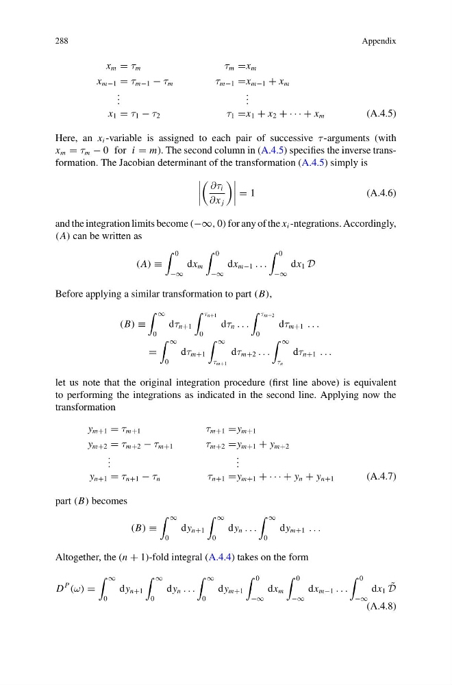
Here, an x i -variable is assigned to each pair of successive τ -arguments (with
x m = τ m − 0 for i = m). The second column in (A.4.5) specifies the inverse transformation. The Jacobian determinant of the transformation (A.4.5) simply is
∂τ i
∂x j
= 1
(A.4.6)
and the integration limits become (−∞, 0) for any of the x i -ntegrations. Accordingly,
(A) can be written as
(A) ≡
0
−∞
dx m
0
−∞
dx m−1 . . .
0
−∞
dx 1 D
Before applying a similar transformation to part (B),
(B) ≡
∞
0
dτ n+1
τ n+1
0
dτ n . . .
τ m+2
0
dτ m+1 . . .
=
∞
0
dτ m+1
∞
τ m+1
dτ m+2 . . .
∞
τ n
dτ n+1 . . .
let us note that the original integration procedure (first line above) is equivalent
to performing the integrations as indicated in the second line. Applying now the
transformation
y m+1 = τ m+1
τ m+1 =y m+1
y m+2 = τ m+2 − τ m+1
τ m+2 =y m+1 + y m+2
. . .
. . .
y n+1 = τ n+1 − τ n
τ n+1 =y m+1 + · · · + y n + y n+1
(A.4.7)
part (B) becomes
(B) ≡
∞
0
dy n+1
∞
0
dy n . . .
∞
0
dy m+1 . . .
Altogether, the (n + 1)-fold integral (A.4.4) takes on the form
D
P
(ω) =
∞
0
dy n+1
∞
0
dy n . . .
∞
0
dy m+1
0
−∞
dx m
0
−∞
dx m−1 . . .
0
−∞
dx 1 ˜
D
(A.4.8)
Appendix
x m = τ m
τ m =x m
x m−1 = τ m−1 − τ m
τ m−1 =x m−1 + x m
. . .
. . .
x 1 = τ 1 − τ 2
τ 1 =x 1 + x 2 + · · · + x m
(A.4.5)
Here, an x i -variable is assigned to each pair of successive τ -arguments (with
x m = τ m − 0 for i = m). The second column in (A.4.5) specifies the inverse transformation. The Jacobian determinant of the transformation (A.4.5) simply is
∂τ i
∂x j
= 1
(A.4.6)
and the integration limits become (−∞, 0) for any of the x i -ntegrations. Accordingly,
(A) can be written as
(A) ≡
0
−∞
dx m
0
−∞
dx m−1 . . .
0
−∞
dx 1 D
Before applying a similar transformation to part (B),
(B) ≡
∞
0
dτ n+1
τ n+1
0
dτ n . . .
τ m+2
0
dτ m+1 . . .
=
∞
0
dτ m+1
∞
τ m+1
dτ m+2 . . .
∞
τ n
dτ n+1 . . .
let us note that the original integration procedure (first line above) is equivalent
to performing the integrations as indicated in the second line. Applying now the
transformation
y m+1 = τ m+1
τ m+1 =y m+1
y m+2 = τ m+2 − τ m+1
τ m+2 =y m+1 + y m+2
. . .
. . .
y n+1 = τ n+1 − τ n
τ n+1 =y m+1 + · · · + y n + y n+1
(A.4.7)
part (B) becomes
(B) ≡
∞
0
dy n+1
∞
0
dy n . . .
∞
0
dy m+1 . . .
Altogether, the (n + 1)-fold integral (A.4.4) takes on the form
D
P
(ω) =
∞
0
dy n+1
∞
0
dy n . . .
∞
0
dy m+1
0
−∞
dx m
0
−∞
dx m−1 . . .
0
−∞
dx 1 ˜
D
(A.4.8)