

280
Appendix
( ˆ
H 0 − E
(0)
0 )| 0 () = −
∞
n=1
(−i)
n−1
n!
0
−∞
dt 1 e
t 1 . . .
0
−∞
dt n e
t n
ˆ
T T T
n
k=1
∂
∂t k
ˆ
H I (t 1 ) ˆ
H I (t 2 ) . . . ˆ
H I (t n )
| 0
(A.2.5)
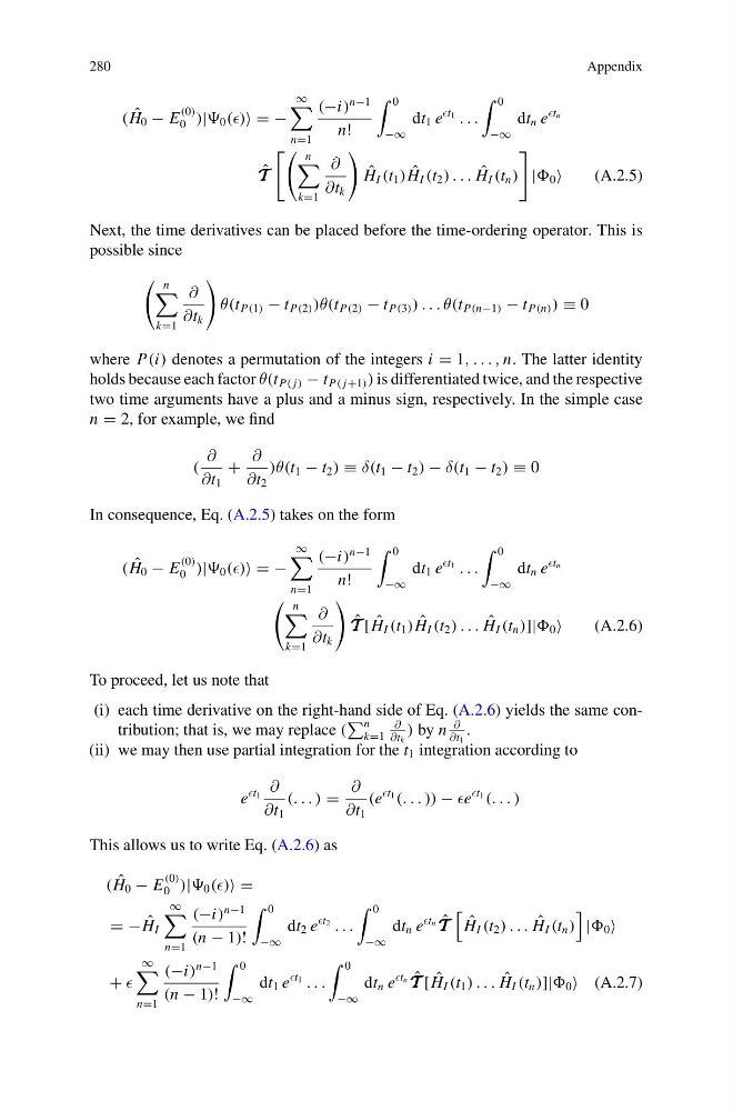
Next, the time derivatives can be placed before the time-ordering operator. This is
possible since
n
k=1
∂
∂t k
θ(t P(1) − t P(2) )θ(t P(2) − t P(3) ) . . . θ(t P(n−1) − t P(n) ) ≡ 0
where P(i) denotes a permutation of the integers i = 1, . . . , n. The latter identity
holds because each factor θ(t P( j) − t P( j+1) ) is differentiated twice, and the respective
two time arguments have a plus and a minus sign, respectively. In the simple case
n = 2, for example, we find
(
∂
∂t 1
+
∂
∂t 2
)θ(t 1 − t 2 ) ≡ δ(t 1 − t 2 ) − δ(t 1 − t 2 ) ≡ 0
In consequence, Eq. (A.2.5) takes on the form
( ˆ
H 0 − E
(0)
0 )| 0 () = −
∞
n=1
(−i)
n−1
n!
0
−∞
dt 1 e
t 1 . . .
0
−∞
dt n e
t n
n
k=1
∂
∂t k
ˆ
T T T [ ˆ
H I (t 1 ) ˆ
H I (t 2 ) . . . ˆ
H I (t n )]| 0
(A.2.6)
To proceed, let us note that
(i) each time derivative on the right-hand side of Eq. (A.2.6) yields the same contribution; that is, we may replace (
n
k=1
∂
∂t k
) by n
∂
∂t 1
.
(ii) we may then use partial integration for the t 1 integration according to
e
t 1
∂
∂t 1
(. . . ) =
∂
∂t 1
(e
t 1 (. . . )) − e
t 1 (. . . )
This allows us to write Eq. (A.2.6) as
( ˆ
H 0 − E
(0)
0 )| 0 () =
= − ˆ
H I
∞
n=1
(−i)
n−1
(n − 1)!
0
−∞
dt 2 e
t 2 . . .
0
−∞
dt n e
t n ˆ
T T T
ˆ
H I (t 2 ) . . . ˆ
H I (t n )
| 0
+
∞
n=1
(−i)
n−1
(n − 1)!
0
−∞
dt 1 e
t 1 . . .
0
−∞
dt n e
t n ˆ
T T T [ ˆ
H I (t 1 ) . . . ˆ
H I (t n )]| 0 (A.2.7)
Appendix
( ˆ
H 0 − E
(0)
0 )| 0 () = −
∞
n=1
(−i)
n−1
n!
0
−∞
dt 1 e
t 1 . . .
0
−∞
dt n e
t n
ˆ
T T T
n
k=1
∂
∂t k
ˆ
H I (t 1 ) ˆ
H I (t 2 ) . . . ˆ
H I (t n )
| 0
(A.2.5)
Next, the time derivatives can be placed before the time-ordering operator. This is
possible since
n
k=1
∂
∂t k
θ(t P(1) − t P(2) )θ(t P(2) − t P(3) ) . . . θ(t P(n−1) − t P(n) ) ≡ 0
where P(i) denotes a permutation of the integers i = 1, . . . , n. The latter identity
holds because each factor θ(t P( j) − t P( j+1) ) is differentiated twice, and the respective
two time arguments have a plus and a minus sign, respectively. In the simple case
n = 2, for example, we find
(
∂
∂t 1
+
∂
∂t 2
)θ(t 1 − t 2 ) ≡ δ(t 1 − t 2 ) − δ(t 1 − t 2 ) ≡ 0
In consequence, Eq. (A.2.5) takes on the form
( ˆ
H 0 − E
(0)
0 )| 0 () = −
∞
n=1
(−i)
n−1
n!
0
−∞
dt 1 e
t 1 . . .
0
−∞
dt n e
t n
n
k=1
∂
∂t k
ˆ
T T T [ ˆ
H I (t 1 ) ˆ
H I (t 2 ) . . . ˆ
H I (t n )]| 0
(A.2.6)
To proceed, let us note that
(i) each time derivative on the right-hand side of Eq. (A.2.6) yields the same contribution; that is, we may replace (
n
k=1
∂
∂t k
) by n
∂
∂t 1
.
(ii) we may then use partial integration for the t 1 integration according to
e
t 1
∂
∂t 1
(. . . ) =
∂
∂t 1
(e
t 1 (. . . )) − e
t 1 (. . . )
This allows us to write Eq. (A.2.6) as
( ˆ
H 0 − E
(0)
0 )| 0 () =
= − ˆ
H I
∞
n=1
(−i)
n−1
(n − 1)!
0
−∞
dt 2 e
t 2 . . .
0
−∞
dt n e
t n ˆ
T T T
ˆ
H I (t 2 ) . . . ˆ
H I (t n )
| 0
+
∞
n=1
(−i)
n−1
(n − 1)!
0
−∞
dt 1 e
t 1 . . .
0
−∞
dt n e
t n ˆ
T T T [ ˆ
H I (t 1 ) . . . ˆ
H I (t n )]| 0 (A.2.7)