

Appendix
279
A.2 Proof of the Gell-Mann and Low Theorem
The proof of the Gell-Mann and Low theorem presented in the following is essentially
based on the version given in the textbook by Fetter and Walecka [5].
Theorem:
If the state
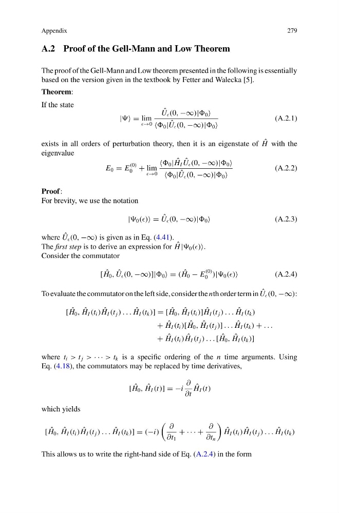
| = lim
→0
ˆ
U (0, −∞)| 0
0 | ˆ
U (0, −∞)| 0
(A.2.1)
exists in all orders of perturbation theory, then it is an eigenstate of ˆ
H with the
eigenvalue
E 0 = E
(0)
0 + lim
→0
0 | ˆ
H I ˆ
U (0, −∞)| 0
0 | ˆ
U (0, −∞)| 0
(A.2.2)
Proof:
For brevity, we use the notation
| 0 () = ˆ
U (0, −∞)| 0
(A.2.3)
where ˆ
U (0, −∞) is given as in Eq. (4.41).
The first step is to derive an expression for ˆ
H | 0 ().
Consider the commutator
[ ˆ
H 0 , ˆ
U (0, −∞)]| 0 = ( ˆ
H 0 − E
(0)
0 )| 0 ()
(A.2.4)
To evaluate the commutator on the left side, consider the nth order term in ˆ
U (0, −∞):
[ ˆ
H 0 , ˆ
H I (t i ) ˆ
H I (t j ) . . . ˆ
H I (t k )] = [ ˆ
H 0 , ˆ
H I (t i )] ˆ
H I (t j ) . . . ˆ
H I (t k )
+ ˆ
H I (t i )[ ˆ
H 0 , ˆ
H I (t j )] . . . ˆ
H I (t k ) + . . .
+ ˆ
H I (t i ) ˆ
H I (t j ) . . . [ ˆ
H 0 , ˆ
H I (t k )]
where t i > t j > · · · > t k is a specific ordering of the n time arguments. Using
Eq. (4.18), the commutators may be replaced by time derivatives,
[ ˆ
H 0 , ˆ
H I (t)] = −i
∂
∂t
ˆ
H I (t)
which yields
[ ˆ
H 0 , ˆ
H I (t i ) ˆ
H I (t j ) . . . ˆ
H I (t k )] = (−i)
∂
∂t 1
+ · · · +
∂
∂t n
ˆ
H I (t i ) ˆ
H I (t j ) . . . ˆ
H I (t k )
This allows us to write the right-hand side of Eq. (A.2.4) in the form
279
A.2 Proof of the Gell-Mann and Low Theorem
The proof of the Gell-Mann and Low theorem presented in the following is essentially
based on the version given in the textbook by Fetter and Walecka [5].
Theorem:
If the state
| = lim
→0
ˆ
U (0, −∞)| 0
0 | ˆ
U (0, −∞)| 0
(A.2.1)
exists in all orders of perturbation theory, then it is an eigenstate of ˆ
H with the
eigenvalue
E 0 = E
(0)
0 + lim
→0
0 | ˆ
H I ˆ
U (0, −∞)| 0
0 | ˆ
U (0, −∞)| 0
(A.2.2)
Proof:
For brevity, we use the notation
| 0 () = ˆ
U (0, −∞)| 0
(A.2.3)
where ˆ
U (0, −∞) is given as in Eq. (4.41).
The first step is to derive an expression for ˆ
H | 0 ().
Consider the commutator
[ ˆ
H 0 , ˆ
U (0, −∞)]| 0 = ( ˆ
H 0 − E
(0)
0 )| 0 ()
(A.2.4)
To evaluate the commutator on the left side, consider the nth order term in ˆ
U (0, −∞):
[ ˆ
H 0 , ˆ
H I (t i ) ˆ
H I (t j ) . . . ˆ
H I (t k )] = [ ˆ
H 0 , ˆ
H I (t i )] ˆ
H I (t j ) . . . ˆ
H I (t k )
+ ˆ
H I (t i )[ ˆ
H 0 , ˆ
H I (t j )] . . . ˆ
H I (t k ) + . . .
+ ˆ
H I (t i ) ˆ
H I (t j ) . . . [ ˆ
H 0 , ˆ
H I (t k )]
where t i > t j > · · · > t k is a specific ordering of the n time arguments. Using
Eq. (4.18), the commutators may be replaced by time derivatives,
[ ˆ
H 0 , ˆ
H I (t)] = −i
∂
∂t
ˆ
H I (t)
which yields
[ ˆ
H 0 , ˆ
H I (t i ) ˆ
H I (t j ) . . . ˆ
H I (t k )] = (−i)
∂
∂t 1
+ · · · +
∂
∂t n
ˆ
H I (t i ) ˆ
H I (t j ) . . . ˆ
H I (t k )
This allows us to write the right-hand side of Eq. (A.2.4) in the form