

278
Appendix
hx = e 0 x
(A.1.43)
where x denotes the ground-state eigenvector. Partitioning of the Schrödinger equation as in Eq. (A.1.32), one obtains the one-dimensional secular equation
e 0 − h 00 − v
†
(e 0 − ˜
h)
−1
v = 0
(A.1.44)
Here, v is the (column) vector of the matrix elements
v k = h k0 = =φ k | ˆ
h 1 |φ 0 , k ≥ 1
(A.1.45)
and ˜
h denotes the sub-block of h with matrix elements h kl , k, l ≥ 1. Writing h 00
more explicitly as h 00 = e
(0)
0 + +φ 0 | ˆ
h 1 |φ 0 and, correspondingly, ˜
h as
˜
h = e
(0)
+ ˜
h 1
(A.1.46)
where e
(0) is the diagonal matrix of eigenvalues e
(0)
k of ˆ
h 0 , k ≥ 1, the one-dimensional
eigenvalue equation (A.1.44) takes on the form
e 0 = e
(0)
0 + +φ 0 | ˆ
h 1 |φ 0 + v
†
(e 0 1 − e
(0)
− ˜
h 1 )
−1
v
(A.1.47)
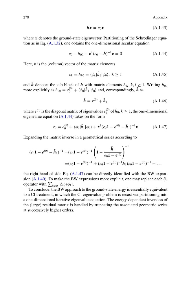
Expanding the matrix inverse in a geometrical series according to
(e 0 1 − e
(0)
− ˜
h 1 )
−1
=(e 0 1 − e
(0)
)
−1
1 −
˜
h 1
e 0 1 − e (0)
−1
=(e 0 1 − e
(0)
)
−1
+ (e 0 1 − e
(0)
)
−1 ˜
h 1 (e 0 1 − e
(0)
)
−1
+ . . .
the right-hand of side Eq. (A.1.47) can be directly identified with the BW expansion (A.1.40). To make the BW expressions more explicit, one may replace each ˆ
q 0
operator with
k =0 |φ k φ k |.
To conclude, the BW approach to the ground-state energy is essentially equivalent
to a CI treatment, in which the CI eigenvalue problem is recast via partitioning into
a one-dimensional iterative eigenvalue equation. The energy-dependent inversion of
the (large) residual matrix is handled by truncating the associated geometric series
at successively higher orders.
Appendix
hx = e 0 x
(A.1.43)
where x denotes the ground-state eigenvector. Partitioning of the Schrödinger equation as in Eq. (A.1.32), one obtains the one-dimensional secular equation
e 0 − h 00 − v
†
(e 0 − ˜
h)
−1
v = 0
(A.1.44)
Here, v is the (column) vector of the matrix elements
v k = h k0 = =φ k | ˆ
h 1 |φ 0 , k ≥ 1
(A.1.45)
and ˜
h denotes the sub-block of h with matrix elements h kl , k, l ≥ 1. Writing h 00
more explicitly as h 00 = e
(0)
0 + +φ 0 | ˆ
h 1 |φ 0 and, correspondingly, ˜
h as
˜
h = e
(0)
+ ˜
h 1
(A.1.46)
where e
(0) is the diagonal matrix of eigenvalues e
(0)
k of ˆ
h 0 , k ≥ 1, the one-dimensional
eigenvalue equation (A.1.44) takes on the form
e 0 = e
(0)
0 + +φ 0 | ˆ
h 1 |φ 0 + v
†
(e 0 1 − e
(0)
− ˜
h 1 )
−1
v
(A.1.47)
Expanding the matrix inverse in a geometrical series according to
(e 0 1 − e
(0)
− ˜
h 1 )
−1
=(e 0 1 − e
(0)
)
−1
1 −
˜
h 1
e 0 1 − e (0)
−1
=(e 0 1 − e
(0)
)
−1
+ (e 0 1 − e
(0)
)
−1 ˜
h 1 (e 0 1 − e
(0)
)
−1
+ . . .
the right-hand of side Eq. (A.1.47) can be directly identified with the BW expansion (A.1.40). To make the BW expressions more explicit, one may replace each ˆ
q 0
operator with
k =0 |φ k φ k |.
To conclude, the BW approach to the ground-state energy is essentially equivalent
to a CI treatment, in which the CI eigenvalue problem is recast via partitioning into
a one-dimensional iterative eigenvalue equation. The energy-dependent inversion of
the (large) residual matrix is handled by truncating the associated geometric series
at successively higher orders.