

Appendix
277
While the relation (A.1.38) is of obvious theoretical interest, one may wonder
about its usefulness in actual computations. Again, this depends on the actual problem
under consideration. If M is a large matrix, full diagonalization is certainly not a
desirable or feasible option. Often, however, one is not interested in the resolvent
matrix as a function of the energy variable, but rather in its particular pole positions,
that is, selected eigenvalues of M. Then, of course the eigenvalue problem of M is
to be dealt with in the first place, and one can resort to the iterative diagonalization
methods such as the Davidson [2] or Lanczos procedures [3, 4]. In case one actually
needs R(ω) as a function of ω such as for frequency-dependent polarizabilities
(see Appendix A.7), a viable computational scheme can be based on the Lanczos
algorithm. There the exact spectral representation according to Eq. (A.1.38) can
be approximated by a corresponding representation in terms of a set of L Lanczos
eigenvalues and eigenvectors (Lanczos pseudo-spectrum), where L is the number of
Lanczos iteration steps.
An Application: Brillouin–Wigner Perturbation Theory
Using the partitioning technique in the eigenvalue problem of the hamiltonian allows
one to understand the essence of the Brillouin–Wigner perturbation theory. The BW
expansion for the ground-state energy is obtained from Eq. (A.1.10) with the choice
= E 0 . For notational ease, we consider the case of a one-particle system, where
that expansion takes on the form
e 0 =e
(0)
0 + +φ 0 | ˆ
h 1 |φ 0 + +φ 0 | ˆ
h 1
∞
ν=1
ˆ
q 0 ˆ
h 1
e 0 − ˆ
h 0
ν
|φ 0
==φ 0 | ˆ
h|φ 0 + +φ 0 | ˆ
h 1
ˆ
q 0
e 0 − ˆ
h 0
ˆ
h 1 |φ 0 + +φ 0 | ˆ
h 1
ˆ
q 0
e 0 − ˆ
h 0
ˆ
h 1
ˆ
q 0
e 0 − ˆ
h 0
ˆ
h 1 |φ 0 + . . .
(A.1.40)
Here, ˆ
q 0 = ˆ
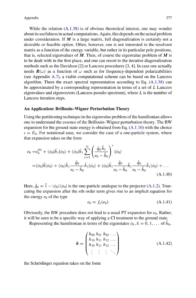
1 − |φ 0 φ 0 | is the one-particle analogue to the projector (A.1.2). Truncating the expansion after the nth order term gives rise to an implicit equation for
the energy e 0 of the type
e 0 = f n (e 0 )
(A.1.41)
Obviously, the BW procedure does not lead to a usual PT expansion for e 0 . Rather,
it will be seen to be a specific way of applying a CI treatment to the ground state.
Representing the hamiltonian in terms of the eigenstates φ k , k = 0, 1, . . . of ˆ
h 0 ,
h =
⎛
⎜
⎜
⎜
⎝
h 00 h 01 h 02 . . .
h 10 h 11 h 12 . . .
h 20 h 21 h 22 . . .
. . .
. . .
. . .
. . .
⎞
⎟
⎟
⎟
⎠
(A.1.42)
the Schrödinger equation takes on the form
277
While the relation (A.1.38) is of obvious theoretical interest, one may wonder
about its usefulness in actual computations. Again, this depends on the actual problem
under consideration. If M is a large matrix, full diagonalization is certainly not a
desirable or feasible option. Often, however, one is not interested in the resolvent
matrix as a function of the energy variable, but rather in its particular pole positions,
that is, selected eigenvalues of M. Then, of course the eigenvalue problem of M is
to be dealt with in the first place, and one can resort to the iterative diagonalization
methods such as the Davidson [2] or Lanczos procedures [3, 4]. In case one actually
needs R(ω) as a function of ω such as for frequency-dependent polarizabilities
(see Appendix A.7), a viable computational scheme can be based on the Lanczos
algorithm. There the exact spectral representation according to Eq. (A.1.38) can
be approximated by a corresponding representation in terms of a set of L Lanczos
eigenvalues and eigenvectors (Lanczos pseudo-spectrum), where L is the number of
Lanczos iteration steps.
An Application: Brillouin–Wigner Perturbation Theory
Using the partitioning technique in the eigenvalue problem of the hamiltonian allows
one to understand the essence of the Brillouin–Wigner perturbation theory. The BW
expansion for the ground-state energy is obtained from Eq. (A.1.10) with the choice
= E 0 . For notational ease, we consider the case of a one-particle system, where
that expansion takes on the form
e 0 =e
(0)
0 + +φ 0 | ˆ
h 1 |φ 0 + +φ 0 | ˆ
h 1
∞
ν=1
ˆ
q 0 ˆ
h 1
e 0 − ˆ
h 0
ν
|φ 0
==φ 0 | ˆ
h|φ 0 + +φ 0 | ˆ
h 1
ˆ
q 0
e 0 − ˆ
h 0
ˆ
h 1 |φ 0 + +φ 0 | ˆ
h 1
ˆ
q 0
e 0 − ˆ
h 0
ˆ
h 1
ˆ
q 0
e 0 − ˆ
h 0
ˆ
h 1 |φ 0 + . . .
(A.1.40)
Here, ˆ
q 0 = ˆ
1 − |φ 0 φ 0 | is the one-particle analogue to the projector (A.1.2). Truncating the expansion after the nth order term gives rise to an implicit equation for
the energy e 0 of the type
e 0 = f n (e 0 )
(A.1.41)
Obviously, the BW procedure does not lead to a usual PT expansion for e 0 . Rather,
it will be seen to be a specific way of applying a CI treatment to the ground state.
Representing the hamiltonian in terms of the eigenstates φ k , k = 0, 1, . . . of ˆ
h 0 ,
h =
⎛
⎜
⎜
⎜
⎝
h 00 h 01 h 02 . . .
h 10 h 11 h 12 . . .
h 20 h 21 h 22 . . .
. . .
. . .
. . .
. . .
⎞
⎟
⎟
⎟
⎠
(A.1.42)
the Schrödinger equation takes on the form