

276
Appendix
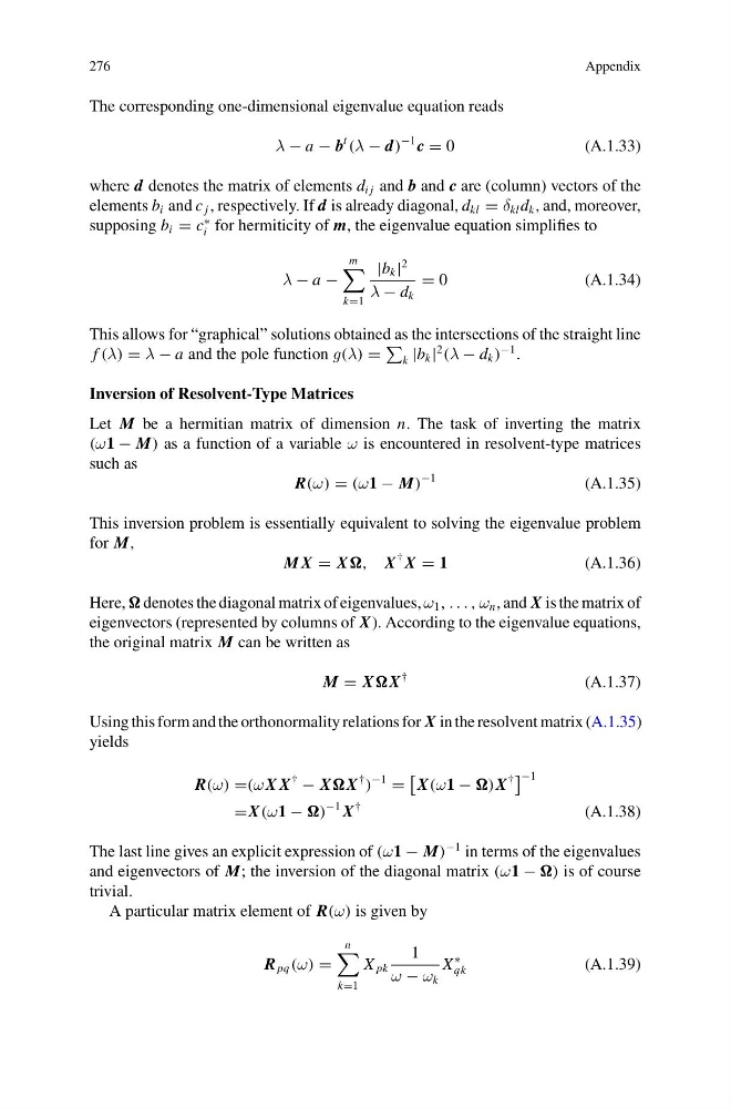
The corresponding one-dimensional eigenvalue equation reads
λ − a − b
t
(λ − d)
−1 c = 0
(A.1.33)
where d denotes the matrix of elements d i j and b and c are (column) vectors of the
elements b i and c j , respectively. If d is already diagonal, d kl = δ kl d k , and, moreover,
supposing b i = c
∗
i for hermiticity of m, the eigenvalue equation simplifies to
λ − a −
m
k=1
|b k |
2
λ − d k
= 0
(A.1.34)
This allows for “graphical” solutions obtained as the intersections of the straight line
f (λ) = λ − a and the pole function g(λ) =
k |b k |
2
(λ − d k )
−1 .
Inversion of Resolvent-Type Matrices
Let M be a hermitian matrix of dimension n. The task of inverting the matrix
(ω1 − M) as a function of a variable ω is encountered in resolvent-type matrices
such as
R(ω) = (ω1 − M)
−1
(A.1.35)
This inversion problem is essentially equivalent to solving the eigenvalue problem
for M,
M X = X, X
† X = 1
(A.1.36)
Here, denotes the diagonal matrix of eigenvalues, ω 1 , . . . , ω n , and X is the matrix of
eigenvectors (represented by columns of X). According to the eigenvalue equations,
the original matrix M can be written as
M = XX
†
(A.1.37)
Using this form and the orthonormality relations for X in the resolvent matrix (A.1.35)
yields
R(ω) =(ω X X
†
− XX
†
)
−1
=
X(ω1 − )X
†
−1
=X(ω1 − )
−1 X
†
(A.1.38)
The last line gives an explicit expression of (ω1 − M)
−1 in terms of the eigenvalues
and eigenvectors of M; the inversion of the diagonal matrix (ω1 − ) is of course
trivial.
A particular matrix element of R(ω) is given by
R pq (ω) =
n
k=1
X pk
1
ω − ω k
X
∗
qk
(A.1.39)
Appendix
The corresponding one-dimensional eigenvalue equation reads
λ − a − b
t
(λ − d)
−1 c = 0
(A.1.33)
where d denotes the matrix of elements d i j and b and c are (column) vectors of the
elements b i and c j , respectively. If d is already diagonal, d kl = δ kl d k , and, moreover,
supposing b i = c
∗
i for hermiticity of m, the eigenvalue equation simplifies to
λ − a −
m
k=1
|b k |
2
λ − d k
= 0
(A.1.34)
This allows for “graphical” solutions obtained as the intersections of the straight line
f (λ) = λ − a and the pole function g(λ) =
k |b k |
2
(λ − d k )
−1 .
Inversion of Resolvent-Type Matrices
Let M be a hermitian matrix of dimension n. The task of inverting the matrix
(ω1 − M) as a function of a variable ω is encountered in resolvent-type matrices
such as
R(ω) = (ω1 − M)
−1
(A.1.35)
This inversion problem is essentially equivalent to solving the eigenvalue problem
for M,
M X = X, X
† X = 1
(A.1.36)
Here, denotes the diagonal matrix of eigenvalues, ω 1 , . . . , ω n , and X is the matrix of
eigenvectors (represented by columns of X). According to the eigenvalue equations,
the original matrix M can be written as
M = XX
†
(A.1.37)
Using this form and the orthonormality relations for X in the resolvent matrix (A.1.35)
yields
R(ω) =(ω X X
†
− XX
†
)
−1
=
X(ω1 − )X
†
−1
=X(ω1 − )
−1 X
†
(A.1.38)
The last line gives an explicit expression of (ω1 − M)
−1 in terms of the eigenvalues
and eigenvectors of M; the inversion of the diagonal matrix (ω1 − ) is of course
trivial.
A particular matrix element of R(ω) is given by
R pq (ω) =
n
k=1
X pk
1
ω − ω k
X
∗
qk
(A.1.39)