

Appendix
275
Here, λ denotes an eigenvalue of M, and the corresponding eigenvector is written in
an obvious partitioned form. More explicitly, the latter equation is composed of the
two sub-block equations
Ax + B y =λx
C x + D y =λ y
coupling the x and y components of the eigenvector. Solving the second equation
for y gives
y = (λ1 − D)
−1 C x
(A.1.30)
which can be used to replace y in the first equation. The result is the following
pseudo-eigenvalue equation for x:
A + B(λ1 − D)
−1 C
x = λx
(A.1.31)
While the matrix on the left-hand side is of smaller dimension than that of the
original matrix M, it depends on the respective eigenvalue λ. This means one has to
resort to an appropriate iterative procedure in order to solve the pseudo-eigenvalue
equation, which of course brings up computational issues such as the convergence
of the procedure to selected (or a manifold of) pseudo-eigenpairs λ k , x k . Once such
an eigenpair has been determined, the y components of the full eigenvector of M
can be obtained using Eq. (A.1.30).
Note that, in general, two pseudo-eigenvectors x k and x l associated with distinct
eigenvalues, λ k = λ l , are not orthogonal. Orthogonality only applies to the full eigenvectors of M, of which the x components are only a part. (As pseudo-eigenvectors
of Eq. (A.1.31) x k and x l derive from distinct sub-block matrices.)
The computational benefit of partitioning the eigenvalue problem depends of
course on the specifics of the problem under consideration. Generally, a partitioning
scheme will be desirable in which the sub-block A is of small dimension and preferably coupled only weakly to the (large) sub-block D via the off-diagonal blocks
B and C (= B
† ). The advantage of a low-dimensional pseudo-eigenvalue problem,
being of the dimension of A, is offset to a certain extent by the need of inverting the
large matrix (λ1 − D) for various values of λ in the iterative procedure. The latter
task is addressed in the following sub-section.
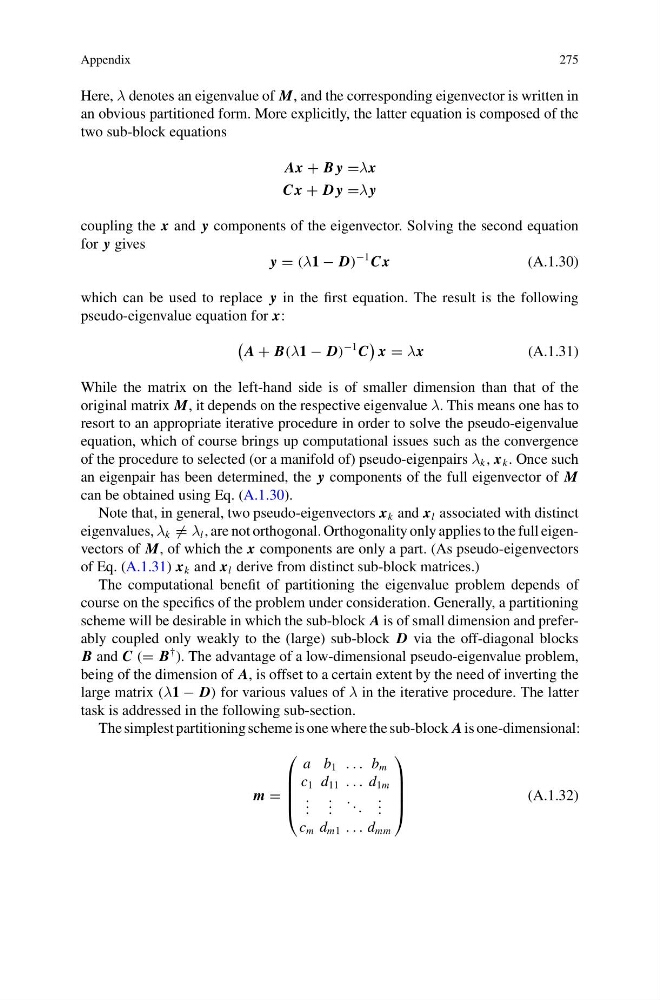
The simplest partitioning scheme is one where the sub-block A is one-dimensional:
m =
⎛
⎜
⎜
⎜
⎝
a b 1 . . . b m
c 1 d 11 . . . d 1m
. . .
. . .
. . .
. . .
c m d m1 . . . d mm
⎞
⎟
⎟
⎟
⎠
(A.1.32)
275
Here, λ denotes an eigenvalue of M, and the corresponding eigenvector is written in
an obvious partitioned form. More explicitly, the latter equation is composed of the
two sub-block equations
Ax + B y =λx
C x + D y =λ y
coupling the x and y components of the eigenvector. Solving the second equation
for y gives
y = (λ1 − D)
−1 C x
(A.1.30)
which can be used to replace y in the first equation. The result is the following
pseudo-eigenvalue equation for x:
A + B(λ1 − D)
−1 C
x = λx
(A.1.31)
While the matrix on the left-hand side is of smaller dimension than that of the
original matrix M, it depends on the respective eigenvalue λ. This means one has to
resort to an appropriate iterative procedure in order to solve the pseudo-eigenvalue
equation, which of course brings up computational issues such as the convergence
of the procedure to selected (or a manifold of) pseudo-eigenpairs λ k , x k . Once such
an eigenpair has been determined, the y components of the full eigenvector of M
can be obtained using Eq. (A.1.30).
Note that, in general, two pseudo-eigenvectors x k and x l associated with distinct
eigenvalues, λ k = λ l , are not orthogonal. Orthogonality only applies to the full eigenvectors of M, of which the x components are only a part. (As pseudo-eigenvectors
of Eq. (A.1.31) x k and x l derive from distinct sub-block matrices.)
The computational benefit of partitioning the eigenvalue problem depends of
course on the specifics of the problem under consideration. Generally, a partitioning
scheme will be desirable in which the sub-block A is of small dimension and preferably coupled only weakly to the (large) sub-block D via the off-diagonal blocks
B and C (= B
† ). The advantage of a low-dimensional pseudo-eigenvalue problem,
being of the dimension of A, is offset to a certain extent by the need of inverting the
large matrix (λ1 − D) for various values of λ in the iterative procedure. The latter
task is addressed in the following sub-section.
The simplest partitioning scheme is one where the sub-block A is one-dimensional:
m =
⎛
⎜
⎜
⎜
⎝
a b 1 . . . b m
c 1 d 11 . . . d 1m
. . .
. . .
. . .
. . .
c m d m1 . . . d mm
⎞
⎟
⎟
⎟
⎠
(A.1.32)