

274
Appendix
has the same block form, and the sub-blocks of the inverse can be directly written in
terms of the original blocks according to
E =( A − B D
−1 C)
−1
,
F = −A
−1 B H
G = − D
−1 C E,
H = ( D − C A
−1 B)
−1
(A.1.27)
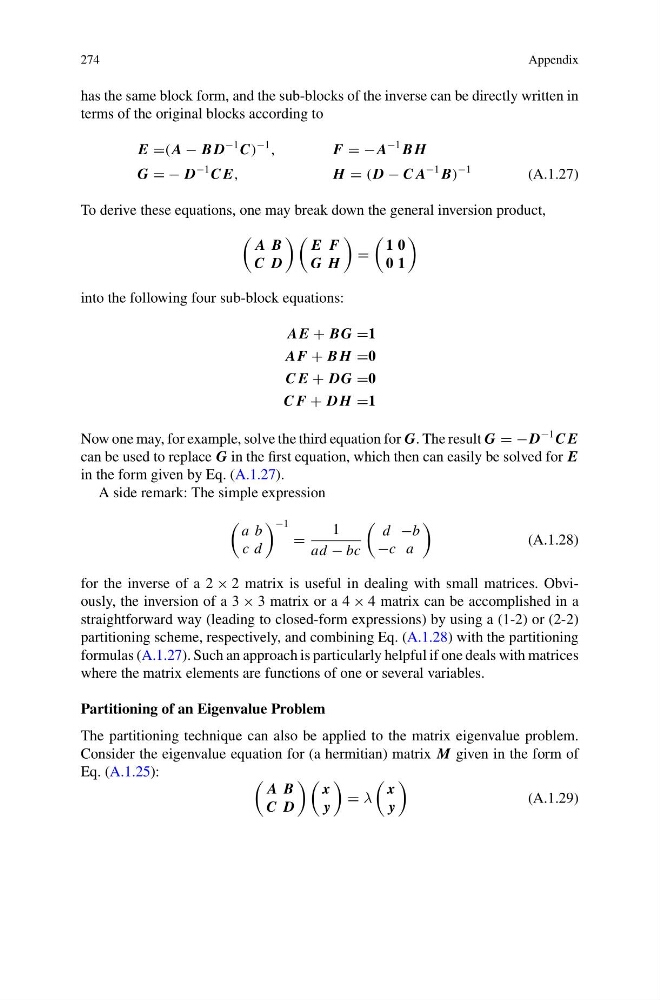
To derive these equations, one may break down the general inversion product,
A B
C D
E F
G H
=
1 0
0 1
into the following four sub-block equations:
AE + BG =1
AF + B H =0
C E + DG =0
C F + D H =1
Now one may, for example, solve the third equation for G. The result G = −D
−1 C E
can be used to replace G in the first equation, which then can easily be solved for E
in the form given by Eq. (A.1.27).
A side remark: The simple expression
a b
c d
−1
=
1
ad − bc
d −b
−c a
(A.1.28)
for the inverse of a 2 × 2 matrix is useful in dealing with small matrices. Obviously, the inversion of a 3 × 3 matrix or a 4 × 4 matrix can be accomplished in a
straightforward way (leading to closed-form expressions) by using a (1-2) or (2-2)
partitioning scheme, respectively, and combining Eq. (A.1.28) with the partitioning
formulas (A.1.27). Such an approach is particularly helpful if one deals with matrices
where the matrix elements are functions of one or several variables.
Partitioning of an Eigenvalue Problem
The partitioning technique can also be applied to the matrix eigenvalue problem.
Consider the eigenvalue equation for (a hermitian) matrix M given in the form of
Eq. (A.1.25):
A B
C D
x
y
= λ
x
y
(A.1.29)
Appendix
has the same block form, and the sub-blocks of the inverse can be directly written in
terms of the original blocks according to
E =( A − B D
−1 C)
−1
,
F = −A
−1 B H
G = − D
−1 C E,
H = ( D − C A
−1 B)
−1
(A.1.27)
To derive these equations, one may break down the general inversion product,
A B
C D
E F
G H
=
1 0
0 1
into the following four sub-block equations:
AE + BG =1
AF + B H =0
C E + DG =0
C F + D H =1
Now one may, for example, solve the third equation for G. The result G = −D
−1 C E
can be used to replace G in the first equation, which then can easily be solved for E
in the form given by Eq. (A.1.27).
A side remark: The simple expression
a b
c d
−1
=
1
ad − bc
d −b
−c a
(A.1.28)
for the inverse of a 2 × 2 matrix is useful in dealing with small matrices. Obviously, the inversion of a 3 × 3 matrix or a 4 × 4 matrix can be accomplished in a
straightforward way (leading to closed-form expressions) by using a (1-2) or (2-2)
partitioning scheme, respectively, and combining Eq. (A.1.28) with the partitioning
formulas (A.1.27). Such an approach is particularly helpful if one deals with matrices
where the matrix elements are functions of one or several variables.
Partitioning of an Eigenvalue Problem
The partitioning technique can also be applied to the matrix eigenvalue problem.
Consider the eigenvalue equation for (a hermitian) matrix M given in the form of
Eq. (A.1.25):
A B
C D
x
y
= λ
x
y
(A.1.29)