

Appendix
281
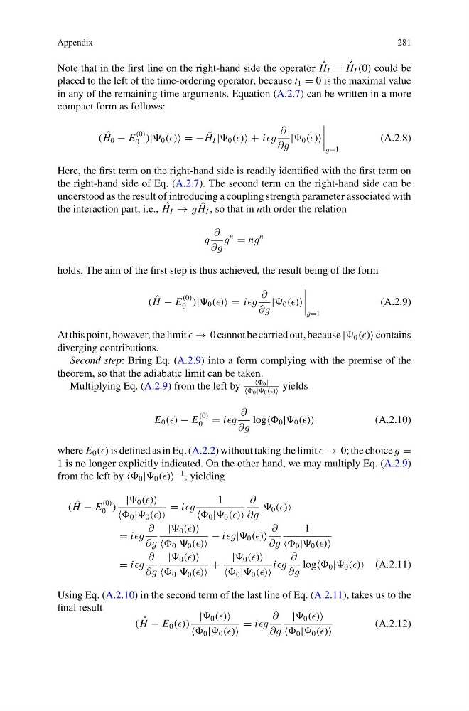
Note that in the first line on the right-hand side the operator ˆ
H I = ˆ
H I (0) could be
placed to the left of the time-ordering operator, because t 1 = 0 is the maximal value
in any of the remaining time arguments. Equation (A.2.7) can be written in a more
compact form as follows:
( ˆ
H 0 − E
(0)
0 )| 0 () = − ˆ
H I | 0 () + ig
∂
∂g
| 0 ()
g=1
(A.2.8)
Here, the first term on the right-hand side is readily identified with the first term on
the right-hand side of Eq. (A.2.7). The second term on the right-hand side can be
understood as the result of introducing a coupling strength parameter associated with
the interaction part, i.e., ˆ
H I → g ˆ
H I , so that in nth order the relation
g
∂
∂g
g
n
= ng
n
holds. The aim of the first step is thus achieved, the result being of the form
( ˆ
H − E
(0)
0 )| 0 () = ig
∂
∂g
| 0 ()
g=1
(A.2.9)
At this point, however, the limit → 0 cannot be carried out, because | 0 () contains
diverging contributions.
Second step: Bring Eq. (A.2.9) into a form complying with the premise of the
theorem, so that the adiabatic limit can be taken.
Multiplying Eq. (A.2.9) from the left by
0 |
0 | 0 ()
yields
E 0 () − E
(0)
0 = ig
∂
∂g
log 0 | 0 ()
(A.2.10)
where E 0 () is defined as in Eq. (A.2.2) without taking the limit → 0; the choice g =
1 is no longer explicitly indicated. On the other hand, we may multiply Eq. (A.2.9)
from the left by 0 | 0 ()
−1 , yielding
( ˆ
H − E
(0)
0 )
| 0 ()
0 | 0 ()
= ig
1
0 | 0 ()
∂
∂g
| 0 ()
= ig
∂
∂g
| 0 ()
0 | 0 ()
− ig| 0 ()
∂
∂g
1
0 | 0 ()
= ig
∂
∂g
| 0 ()
0 | 0 ()
+
| 0 ()
0 | 0 ()
ig
∂
∂g
log 0 | 0 () (A.2.11)
Using Eq. (A.2.10) in the second term of the last line of Eq. (A.2.11), takes us to the
final result
( ˆ
H − E 0 ())
| 0 ()
0 | 0 ()
= ig
∂
∂g
| 0 ()
0 | 0 ()
(A.2.12)
281
Note that in the first line on the right-hand side the operator ˆ
H I = ˆ
H I (0) could be
placed to the left of the time-ordering operator, because t 1 = 0 is the maximal value
in any of the remaining time arguments. Equation (A.2.7) can be written in a more
compact form as follows:
( ˆ
H 0 − E
(0)
0 )| 0 () = − ˆ
H I | 0 () + ig
∂
∂g
| 0 ()
g=1
(A.2.8)
Here, the first term on the right-hand side is readily identified with the first term on
the right-hand side of Eq. (A.2.7). The second term on the right-hand side can be
understood as the result of introducing a coupling strength parameter associated with
the interaction part, i.e., ˆ
H I → g ˆ
H I , so that in nth order the relation
g
∂
∂g
g
n
= ng
n
holds. The aim of the first step is thus achieved, the result being of the form
( ˆ
H − E
(0)
0 )| 0 () = ig
∂
∂g
| 0 ()
g=1
(A.2.9)
At this point, however, the limit → 0 cannot be carried out, because | 0 () contains
diverging contributions.
Second step: Bring Eq. (A.2.9) into a form complying with the premise of the
theorem, so that the adiabatic limit can be taken.
Multiplying Eq. (A.2.9) from the left by
0 |
0 | 0 ()
yields
E 0 () − E
(0)
0 = ig
∂
∂g
log 0 | 0 ()
(A.2.10)
where E 0 () is defined as in Eq. (A.2.2) without taking the limit → 0; the choice g =
1 is no longer explicitly indicated. On the other hand, we may multiply Eq. (A.2.9)
from the left by 0 | 0 ()
−1 , yielding
( ˆ
H − E
(0)
0 )
| 0 ()
0 | 0 ()
= ig
1
0 | 0 ()
∂
∂g
| 0 ()
= ig
∂
∂g
| 0 ()
0 | 0 ()
− ig| 0 ()
∂
∂g
1
0 | 0 ()
= ig
∂
∂g
| 0 ()
0 | 0 ()
+
| 0 ()
0 | 0 ()
ig
∂
∂g
log 0 | 0 () (A.2.11)
Using Eq. (A.2.10) in the second term of the last line of Eq. (A.2.11), takes us to the
final result
( ˆ
H − E 0 ())
| 0 ()
0 | 0 ()
= ig
∂
∂g
| 0 ()
0 | 0 ()
(A.2.12)