

270
Appendix
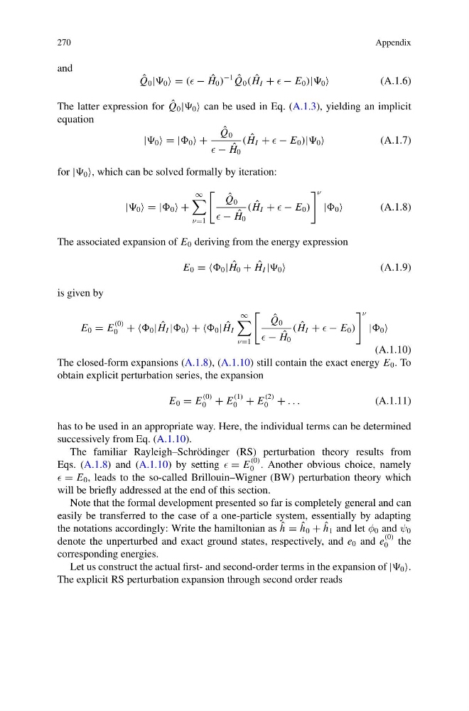
and
ˆ
Q 0 | 0 = ( − ˆ
H 0 )
−1 ˆ
Q 0 ( ˆ
H I + − E 0 )| 0
(A.1.6)
The latter expression for ˆ
Q 0 | 0 can be used in Eq. (A.1.3), yielding an implicit
equation
| 0 = | 0 +
ˆ
Q 0
− ˆ
H 0
( ˆ
H I + − E 0 )| 0
(A.1.7)
for | 0 , which can be solved formally by iteration:
| 0 = | 0 +
∞
ν=1
ˆ
Q 0
− ˆ
H 0
( ˆ
H I + − E 0 )
ν
| 0
(A.1.8)
The associated expansion of E 0 deriving from the energy expression
E 0 = = 0 | ˆ
H 0 + ˆ
H I | 0
(A.1.9)
is given by
E 0 = E
(0)
0 + + 0 | ˆ
H I | 0 + + 0 | ˆ
H I
∞
ν=1
ˆ
Q 0
− ˆ
H 0
( ˆ
H I + − E 0 )
ν
| 0
(A.1.10)
The closed-form expansions (A.1.8), (A.1.10) still contain the exact energy E 0 . To
obtain explicit perturbation series, the expansion
E 0 = E
(0)
0 + E
(1)
0 + E
(2)
0 + . . .
(A.1.11)
has to be used in an appropriate way. Here, the individual terms can be determined
successively from Eq. (A.1.10).
The familiar Rayleigh–Schrödinger (RS) perturbation theory results from
Eqs. (A.1.8) and (A.1.10) by setting = E
(0)
0 . Another obvious choice, namely
= E 0 , leads to the so-called Brillouin–Wigner (BW) perturbation theory which
will be briefly addressed at the end of this section.
Note that the formal development presented so far is completely general and can
easily be transferred to the case of a one-particle system, essentially by adapting
the notations accordingly: Write the hamiltonian as ˆ
h = ˆ
h 0 + ˆ
h 1 and let φ 0 and ψ 0
denote the unperturbed and exact ground states, respectively, and e 0 and e
(0)
0 the
corresponding energies.
Let us construct the actual first- and second-order terms in the expansion of | 0 .
The explicit RS perturbation expansion through second order reads
Appendix
and
ˆ
Q 0 | 0 = ( − ˆ
H 0 )
−1 ˆ
Q 0 ( ˆ
H I + − E 0 )| 0
(A.1.6)
The latter expression for ˆ
Q 0 | 0 can be used in Eq. (A.1.3), yielding an implicit
equation
| 0 = | 0 +
ˆ
Q 0
− ˆ
H 0
( ˆ
H I + − E 0 )| 0
(A.1.7)
for | 0 , which can be solved formally by iteration:
| 0 = | 0 +
∞
ν=1
ˆ
Q 0
− ˆ
H 0
( ˆ
H I + − E 0 )
ν
| 0
(A.1.8)
The associated expansion of E 0 deriving from the energy expression
E 0 = = 0 | ˆ
H 0 + ˆ
H I | 0
(A.1.9)
is given by
E 0 = E
(0)
0 + + 0 | ˆ
H I | 0 + + 0 | ˆ
H I
∞
ν=1
ˆ
Q 0
− ˆ
H 0
( ˆ
H I + − E 0 )
ν
| 0
(A.1.10)
The closed-form expansions (A.1.8), (A.1.10) still contain the exact energy E 0 . To
obtain explicit perturbation series, the expansion
E 0 = E
(0)
0 + E
(1)
0 + E
(2)
0 + . . .
(A.1.11)
has to be used in an appropriate way. Here, the individual terms can be determined
successively from Eq. (A.1.10).
The familiar Rayleigh–Schrödinger (RS) perturbation theory results from
Eqs. (A.1.8) and (A.1.10) by setting = E
(0)
0 . Another obvious choice, namely
= E 0 , leads to the so-called Brillouin–Wigner (BW) perturbation theory which
will be briefly addressed at the end of this section.
Note that the formal development presented so far is completely general and can
easily be transferred to the case of a one-particle system, essentially by adapting
the notations accordingly: Write the hamiltonian as ˆ
h = ˆ
h 0 + ˆ
h 1 and let φ 0 and ψ 0
denote the unperturbed and exact ground states, respectively, and e 0 and e
(0)
0 the
corresponding energies.
Let us construct the actual first- and second-order terms in the expansion of | 0 .
The explicit RS perturbation expansion through second order reads