

212
14 ADC and ISR Approaches to the Polarization Propagator
where
C
(A)
ak,a k =
1
2
δ kk
c,i, j
v aci j v i ja c
i + j − c −
1
2
(( a + a )
(14.37)
C
(B)
ak,a k =
1
2
δ aa
c,d,i
v cdki v k icd
1
2
(( k + k ) + i − c − d
(14.38)
C
(C)
ak,a k =
c,i
v k ia c v acik
1
2
(( k + k − a − a ) + i − c
(14.39)
using again the abbreviations v rsuv as defined in Eq. (10.31).
1 p -1h/2 p -2h coupling block:
C
(1)
ak,a b k l = δ aa V k l [kb ] − δ ab V k l [ka ] − δ kk V al [a b ] + δ kl V ak [a b ]
(14.40)
2 p-2h block:
K abkl,a b k l = (( a + b − k − l )δ aa δ bb δ kk δ ll
(14.41)
The relative signs have been chosen such that the first-order contributions C
(1)
I J are
consistent with I | ˆ
H I − E 0 (1)| J . The ADC(2) expressions for the transition
amplitudes f
(0−2)
1
and f
(1)
2 are listed in Appendix A.9.
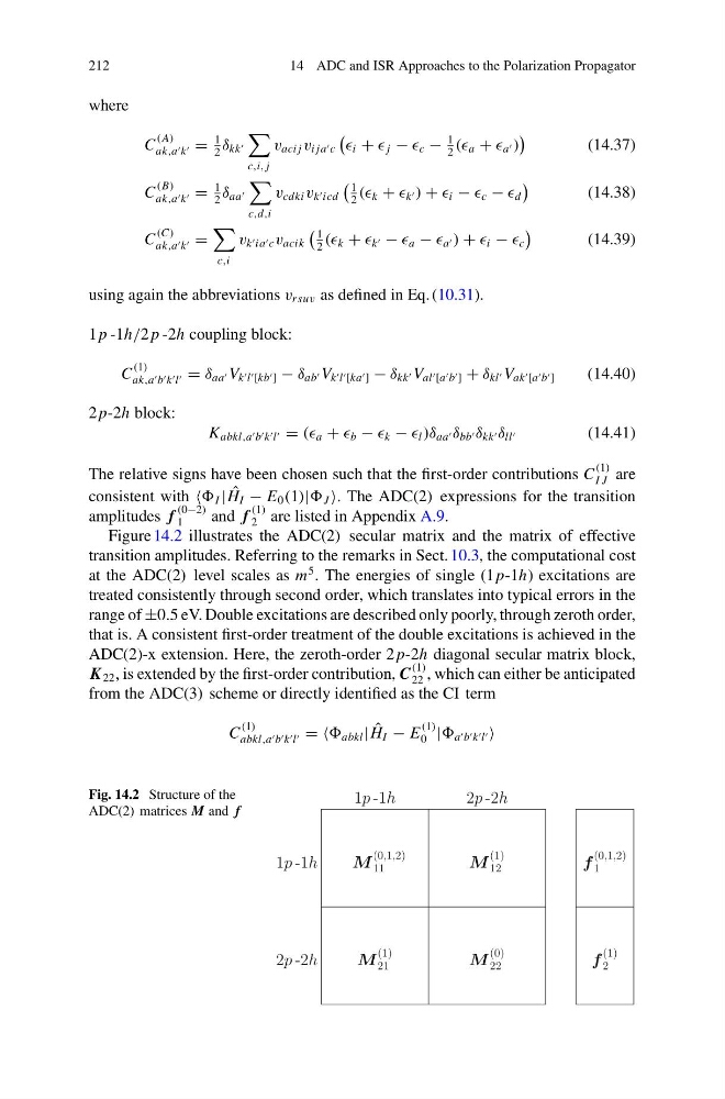
Figure 14.2 illustrates the ADC(2) secular matrix and the matrix of effective
transition amplitudes. Referring to the remarks in Sect. 10.3, the computational cost
at the ADC(2) level scales as m
5 . The energies of single (1 p-1h) excitations are
treated consistently through second order, which translates into typical errors in the
range of ±0.5 eV. Double excitations are described only poorly, through zeroth order,
that is. A consistent first-order treatment of the double excitations is achieved in the
ADC(2)-x extension. Here, the zeroth-order 2 p-2h diagonal secular matrix block,
K 22 , is extended by the first-order contribution, C
(1)
22 , which can either be anticipated
from the ADC(3) scheme or directly identified as the CI term
C
(1)
abkl,a b k l = = abkl | ˆ
H I − E
(1)
0 | a b k l
Fig. 14.2 Structure of the
ADC(2) matrices M and f
1p -1h
2p -2h
1p -1h
M
(0,1,2)
11
M
(1)
12
2p -2h
M
(1)
21
M
(0)
22
f
(0,1,2)
1
f
(1)
2
14 ADC and ISR Approaches to the Polarization Propagator
where
C
(A)
ak,a k =
1
2
δ kk
c,i, j
v aci j v i ja c
i + j − c −
1
2
(( a + a )
(14.37)
C
(B)
ak,a k =
1
2
δ aa
c,d,i
v cdki v k icd
1
2
(( k + k ) + i − c − d
(14.38)
C
(C)
ak,a k =
c,i
v k ia c v acik
1
2
(( k + k − a − a ) + i − c
(14.39)
using again the abbreviations v rsuv as defined in Eq. (10.31).
1 p -1h/2 p -2h coupling block:
C
(1)
ak,a b k l = δ aa V k l [kb ] − δ ab V k l [ka ] − δ kk V al [a b ] + δ kl V ak [a b ]
(14.40)
2 p-2h block:
K abkl,a b k l = (( a + b − k − l )δ aa δ bb δ kk δ ll
(14.41)
The relative signs have been chosen such that the first-order contributions C
(1)
I J are
consistent with I | ˆ
H I − E 0 (1)| J . The ADC(2) expressions for the transition
amplitudes f
(0−2)
1
and f
(1)
2 are listed in Appendix A.9.
Figure 14.2 illustrates the ADC(2) secular matrix and the matrix of effective
transition amplitudes. Referring to the remarks in Sect. 10.3, the computational cost
at the ADC(2) level scales as m
5 . The energies of single (1 p-1h) excitations are
treated consistently through second order, which translates into typical errors in the
range of ±0.5 eV. Double excitations are described only poorly, through zeroth order,
that is. A consistent first-order treatment of the double excitations is achieved in the
ADC(2)-x extension. Here, the zeroth-order 2 p-2h diagonal secular matrix block,
K 22 , is extended by the first-order contribution, C
(1)
22 , which can either be anticipated
from the ADC(3) scheme or directly identified as the CI term
C
(1)
abkl,a b k l = = abkl | ˆ
H I − E
(1)
0 | a b k l
Fig. 14.2 Structure of the
ADC(2) matrices M and f
1p -1h
2p -2h
1p -1h
M
(0,1,2)
11
M
(1)
12
2p -2h
M
(1)
21
M
(0)
22
f
(0,1,2)
1
f
(1)
2