

14.2 Explicit ADC Schemes for the Polarization Propagator
211
(1)
(2)
(3)
(4)
(5)
(6)
(7)
(8)
(9)
(10)
(11)
(12)
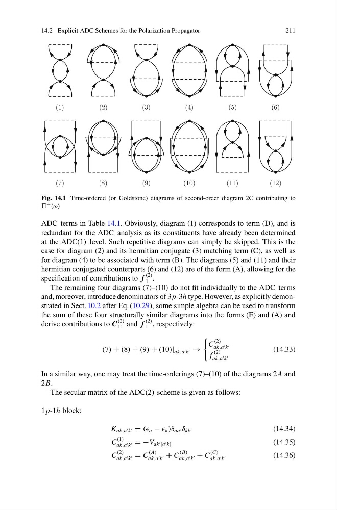
Fig. 14.1 Time-ordered (or Goldstone) diagrams of second-order diagram 2C contributing to
+ (ω)
ADC terms in Table 14.1. Obviously, diagram (1) corresponds to term (D), and is
redundant for the ADC analysis as its constituents have already been determined
at the ADC(1) level. Such repetitive diagrams can simply be skipped. This is the
case for diagram (2) and its hermitian conjugate (3) matching term (C), as well as
for diagram (4) to be associated with term (B). The diagrams (5) and (11) and their
hermitian conjugated counterparts (6) and (12) are of the form (A), allowing for the
specification of contributions to f
(2)
1 .
The remaining four diagrams (7)–(10) do not fit individually to the ADC terms
and, moreover, introduce denominators of 3 p-3h type. However, as explicitly demonstrated in Sect. 10.2 after Eq. (10.29), some simple algebra can be used to transform
the sum of these four structurally similar diagrams into the forms (E) and (A) and
derive contributions to C
(2)
11 and f
(2)
1 , respectively:
(7) + (8) + (9) + (10)| ak,a k →
C
(2)
ak,a k
f
(2)
ak,a k
(14.33)
In a similar way, one may treat the time-orderings (7)–(10) of the diagrams 2 A and
2B.
The secular matrix of the ADC(2) scheme is given as follows:
1 p-1h block:
K ak,a k = (( a − k )δ aa δ kk
(14.34)
C
(1)
ak,a k = −V ak [a k]
(14.35)
C
(2)
ak,a k = C
(A)
ak,a k + C
(B)
ak,a k + C
(C)
ak,a k
(14.36)
211
(1)
(2)
(3)
(4)
(5)
(6)
(7)
(8)
(9)
(10)
(11)
(12)
Fig. 14.1 Time-ordered (or Goldstone) diagrams of second-order diagram 2C contributing to
+ (ω)
ADC terms in Table 14.1. Obviously, diagram (1) corresponds to term (D), and is
redundant for the ADC analysis as its constituents have already been determined
at the ADC(1) level. Such repetitive diagrams can simply be skipped. This is the
case for diagram (2) and its hermitian conjugate (3) matching term (C), as well as
for diagram (4) to be associated with term (B). The diagrams (5) and (11) and their
hermitian conjugated counterparts (6) and (12) are of the form (A), allowing for the
specification of contributions to f
(2)
1 .
The remaining four diagrams (7)–(10) do not fit individually to the ADC terms
and, moreover, introduce denominators of 3 p-3h type. However, as explicitly demonstrated in Sect. 10.2 after Eq. (10.29), some simple algebra can be used to transform
the sum of these four structurally similar diagrams into the forms (E) and (A) and
derive contributions to C
(2)
11 and f
(2)
1 , respectively:
(7) + (8) + (9) + (10)| ak,a k →
C
(2)
ak,a k
f
(2)
ak,a k
(14.33)
In a similar way, one may treat the time-orderings (7)–(10) of the diagrams 2 A and
2B.
The secular matrix of the ADC(2) scheme is given as follows:
1 p-1h block:
K ak,a k = (( a − k )δ aa δ kk
(14.34)
C
(1)
ak,a k = −V ak [a k]
(14.35)
C
(2)
ak,a k = C
(A)
ak,a k + C
(B)
ak,a k + C
(C)
ak,a k
(14.36)