168
11 Intermediate-State Representation (ISR)
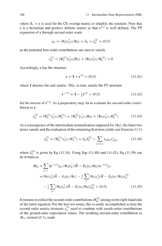
where S 1 = s is used for the CE overlap matrix to simplify the notation. Note that
s is a hermitian and positive definite matrix so that s
1/2 is well defined. The PT
expansion of s through second order reads
s kl = = 0 |c
†
k c l | 0 = δ kl + s
(2)
kl + O(3)
as the potential first-order contributions are seen to vanish,
s
(1)
kl = =
(1)
0 |c
†
k c l | 0 + + 0 |c
†
k c l |
(1)
0 = 0
Accordingly, s has the structure
s = 1 + s
(2)
+ O(3)
(11.41)
where 1 denotes the unit matrix. This, in turn, entails the PT structure
s
−1/2
= 1 −
1
2
s
(2)
+ O(3)
(11.42)
for the inverse of s
1/2 . As a preparatory step, let us evaluate the second-order contribution to s:
s
(2)
kl = =
(1)
0 |c
†
k c l |
(1)
0 + +
(2)
0 |c
†
k c l | 0 + + 0 |c
†
k c l |
(2)
0
(11.43)
As a consequence of the intermediate normalization supposed for | 0 , the latter two
terms vanish, and the evaluation of the remaining first term yields (see Exercise 11.1)
s
(2)
kl = =
(1)
0 |c
†
k c l |
(1)
0 = δ kl I
(2)
0 −
a v abk j v
∗
abl j
(11.44)
where I
(2)
0 is given by Eq. (11.34). Using Eqs. (11.40) and (11.42), Eq. (11.39) can
be written as
M kl =
k ,l
(s
−1/2
) kk 0 |c
†
k ( ˆ
H − E 0 )c l | 0 (s
−1/2
) l l
== 0 |c
†
k ( ˆ
H − E 0 )c l | 0 −
1
2
l
0 |c
†
k ( ˆ
H − E 0 )c l | 0 s
(2)
l l
−
1
2
k
0 |c
†
k ( ˆ
H − E 0 )c l | 0 s
(2)
kk + O(3)
(11.45)
It remains to collect the second-order contributions M
(2)
kl arising on the right-hand side
of the latter equation. For the last two terms, this is easily accomplished as here the
second-order matrix elements s
(2)
i j need to combine with zeroth-order contributions
of the ground-state expectation values. The resulting second-order contribution to
M kl , termed (C1), reads