

11.2 Explicit ISR Procedure Through Second Order
169
(C1) ≡
1
2
( k + l )s
(2)
kl
(11.46)
with s
(2)
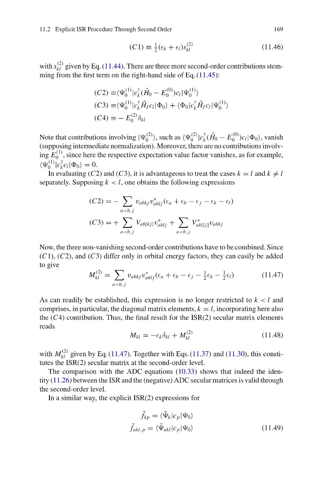
kl given by Eq. (11.44). There are three more second-order contributions stemming from the first term on the right-hand side of Eq. (11.45):
(C2) ≡≡
(1)
0 |c
†
k ( ˆ
H 0 − E
(0)
0 )c l |
(1)
0
(C3) ≡≡
(1)
0 |c
†
k
ˆ
H I c l | 0 + + 0 |c
†
k
ˆ
H I c l |
(1)
0
(C4) ≡ − E
(2)
0 δ kl
Note that contributions involving |
(2)
0 , such as
(2)
0 |c
†
k ( ˆ
H 0 − E
(0)
0 )c l | 0 , vanish
(supposing intermediate normalization). Moreover, there are no contributions involving E
(1)
0 , since here the respective expectation value factor vanishes, as for example,
(1)
0 |c
†
k c l | 0 = 0.
In evaluating (C2) and (C3), it is advantageous to treat the cases k = l and k = l
separately. Supposing k < l, one obtains the following expressions
(C2) = −
a
∗
abl j ( a + b − j − k − l )
(C3) = +
a
∗
abl j +
a
∗
ab[l j] v abk j
Now, the three non-vanishing second-order contributions have to be combined. Since
(C1), (C2), and (C3) differ only in orbital energy factors, they can easily be added
to give
M
(2)
kl =
a
∗
abl j ( a + b − j −
1
2
k −
1
2
l )
(11.47)
As can readily be established, this expression is no longer restricted to k < l and
comprises, in particular, the diagonal matrix elements, k = l, incorporating here also
the (C4) contribution. Thus, the final result for the ISR(2) secular matrix elements
reads
M kl = − k δ kl + M
(2)
kl
(11.48)
with M
(2)
kl given by Eq. (11.47). Together with Eqs. (11.37) and (11.30), this constitutes the ISR(2) secular matrix at the second-order level.
The comparison with the ADC equations (10.33) shows that indeed the identity (11.26) between the ISR and the (negative) ADC secular matrices is valid through
the second-order level.
In a similar way, the explicit ISR(2) expressions for
˜
f kp = = ˜
k |c p | 0
˜
f akl, p = = ˜
akl |c p | 0
(11.49)
169
(C1) ≡
1
2
( k + l )s
(2)
kl
(11.46)
with s
(2)
kl given by Eq. (11.44). There are three more second-order contributions stemming from the first term on the right-hand side of Eq. (11.45):
(C2) ≡≡
(1)
0 |c
†
k ( ˆ
H 0 − E
(0)
0 )c l |
(1)
0
(C3) ≡≡
(1)
0 |c
†
k
ˆ
H I c l | 0 + + 0 |c
†
k
ˆ
H I c l |
(1)
0
(C4) ≡ − E
(2)
0 δ kl
Note that contributions involving |
(2)
0 , such as
(2)
0 |c
†
k ( ˆ
H 0 − E
(0)
0 )c l | 0 , vanish
(supposing intermediate normalization). Moreover, there are no contributions involving E
(1)
0 , since here the respective expectation value factor vanishes, as for example,
(1)
0 |c
†
k c l | 0 = 0.
In evaluating (C2) and (C3), it is advantageous to treat the cases k = l and k = l
separately. Supposing k < l, one obtains the following expressions
(C2) = −
a
∗
abl j ( a + b − j − k − l )
(C3) = +
a
∗
abl j +
a
∗
ab[l j] v abk j
Now, the three non-vanishing second-order contributions have to be combined. Since
(C1), (C2), and (C3) differ only in orbital energy factors, they can easily be added
to give
M
(2)
kl =
a
∗
abl j ( a + b − j −
1
2
k −
1
2
l )
(11.47)
As can readily be established, this expression is no longer restricted to k < l and
comprises, in particular, the diagonal matrix elements, k = l, incorporating here also
the (C4) contribution. Thus, the final result for the ISR(2) secular matrix elements
reads
M kl = − k δ kl + M
(2)
kl
(11.48)
with M
(2)
kl given by Eq. (11.47). Together with Eqs. (11.37) and (11.30), this constitutes the ISR(2) secular matrix at the second-order level.
The comparison with the ADC equations (10.33) shows that indeed the identity (11.26) between the ISR and the (negative) ADC secular matrices is valid through
the second-order level.
In a similar way, the explicit ISR(2) expressions for
˜
f kp = = ˜
k |c p | 0
˜
f akl, p = = ˜
akl |c p | 0
(11.49)