

11.2 Explicit ISR Procedure Through Second Order
167
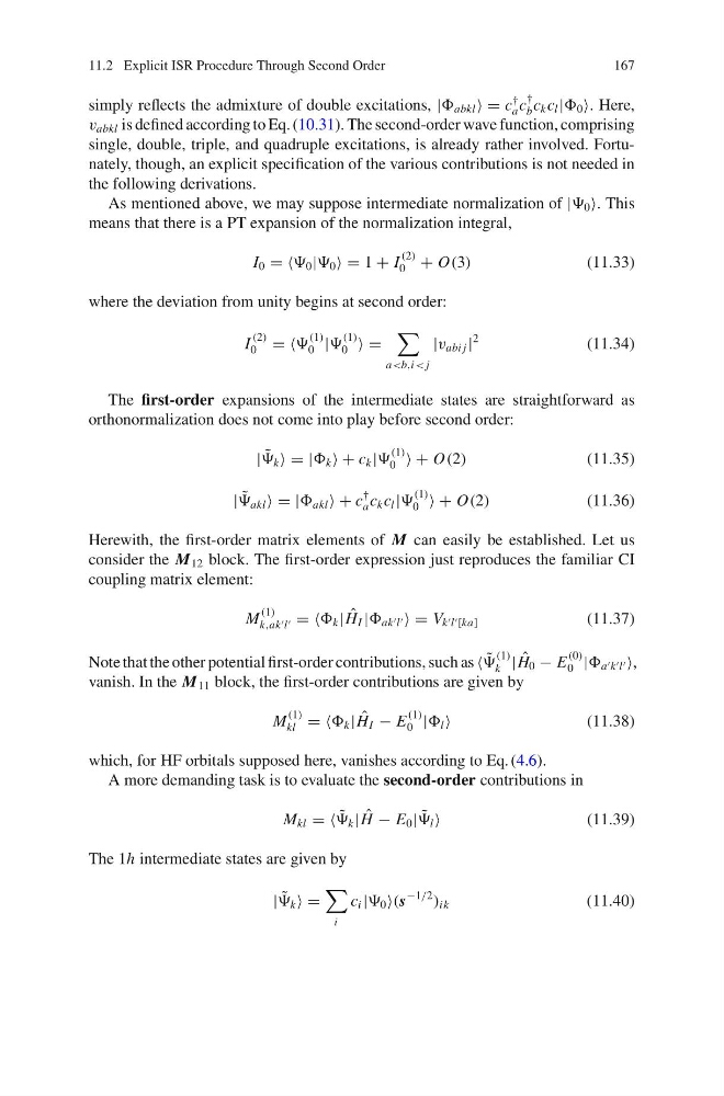
simply reflects the admixture of double excitations, | abkl = c
†
a c
†
b c k c l | 0 . Here,
v abkl is defined according to Eq. (10.31). The second-order wave function, comprising
single, double, triple, and quadruple excitations, is already rather involved. Fortunately, though, an explicit specification of the various contributions is not needed in
the following derivations.
As mentioned above, we may suppose intermediate normalization of | 0 . This
means that there is a PT expansion of the normalization integral,
I 0 = = 0 | 0 = 1 + I
(2)
0 + O(3)
(11.33)
where the deviation from unity begins at second order:
I
(2)
0 = =
(1)
0 |
(1)
0 =
a
2
(11.34)
The first-order expansions of the intermediate states are straightforward as
orthonormalization does not come into play before second order:
| ˜
k = | k + c k |
(1)
0 + O(2)
(11.35)
| ˜
akl = | akl + c
†
a c k c l |
(1)
0 + O(2)
(11.36)
Herewith, the first-order matrix elements of M can easily be established. Let us
consider the M 12 block. The first-order expression just reproduces the familiar CI
coupling matrix element:
M
(1)
k,ak l = = k | ˆ
H I | ak l = V k l [ka]
(11.37)
Note that the other potential first-order contributions, such as ˜
(1)
k | ˆ
H 0 − E
(0)
0 | a k l ,
vanish. In the M 11 block, the first-order contributions are given by
M
(1)
kl = = k | ˆ
H I − E
(1)
0 | l
(11.38)
which, for HF orbitals supposed here, vanishes according to Eq. (4.6).
A more demanding task is to evaluate the second-order contributions in
M kl = = ˜
k | ˆ
H − E 0 | ˜
l
(11.39)
The 1h intermediate states are given by
| ˜
k =
i
c i | 0 (s
−1/2
) ik
(11.40)
167
simply reflects the admixture of double excitations, | abkl = c
†
a c
†
b c k c l | 0 . Here,
v abkl is defined according to Eq. (10.31). The second-order wave function, comprising
single, double, triple, and quadruple excitations, is already rather involved. Fortunately, though, an explicit specification of the various contributions is not needed in
the following derivations.
As mentioned above, we may suppose intermediate normalization of | 0 . This
means that there is a PT expansion of the normalization integral,
I 0 = = 0 | 0 = 1 + I
(2)
0 + O(3)
(11.33)
where the deviation from unity begins at second order:
I
(2)
0 = =
(1)
0 |
(1)
0 =
a
2
(11.34)
The first-order expansions of the intermediate states are straightforward as
orthonormalization does not come into play before second order:
| ˜
k = | k + c k |
(1)
0 + O(2)
(11.35)
| ˜
akl = | akl + c
†
a c k c l |
(1)
0 + O(2)
(11.36)
Herewith, the first-order matrix elements of M can easily be established. Let us
consider the M 12 block. The first-order expression just reproduces the familiar CI
coupling matrix element:
M
(1)
k,ak l = = k | ˆ
H I | ak l = V k l [ka]
(11.37)
Note that the other potential first-order contributions, such as ˜
(1)
k | ˆ
H 0 − E
(0)
0 | a k l ,
vanish. In the M 11 block, the first-order contributions are given by
M
(1)
kl = = k | ˆ
H I − E
(1)
0 | l
(11.38)
which, for HF orbitals supposed here, vanishes according to Eq. (4.6).
A more demanding task is to evaluate the second-order contributions in
M kl = = ˜
k | ˆ
H − E 0 | ˜
l
(11.39)
The 1h intermediate states are given by
| ˜
k =
i
c i | 0 (s
−1/2
) ik
(11.40)