

9.2 Dyson-ADC Secular Equations
141
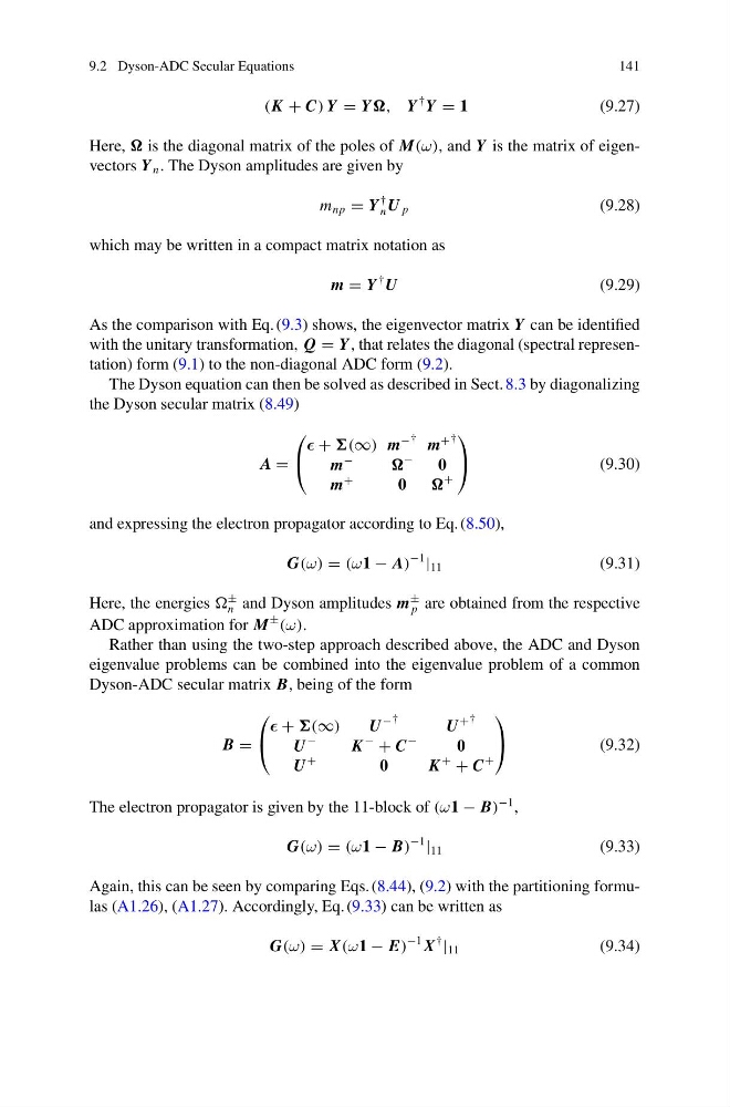
(K + C) Y = Y , Y
† Y = 1
(9.27)
Here, is the diagonal matrix of the poles of M(ω), and Y is the matrix of eigenvectors Y n . The Dyson amplitudes are given by
m np = Y
†
n U p
(9.28)
which may be written in a compact matrix notation as
m = Y
† U
(9.29)
As the comparison with Eq. (9.3) shows, the eigenvector matrix Y can be identified
with the unitary transformation, Q = Y , that relates the diagonal (spectral representation) form (9.1) to the non-diagonal ADC form (9.2).
The Dyson equation can then be solved as described in Sect. 8.3 by diagonalizing
the Dyson secular matrix (8.49)
A =
⎛
⎝
+ (∞) m
− † m
+ †
m
−
−
0
m
+
0
+
⎞
⎠
(9.30)
and expressing the electron propagator according to Eq. (8.50),
G(ω) = (ω1 − A)
−1
| 11
(9.31)
Here, the energies
±
n and Dyson amplitudes m
±
p are obtained from the respective
ADC approximation for M
±
(ω).
Rather than using the two-step approach described above, the ADC and Dyson
eigenvalue problems can be combined into the eigenvalue problem of a common
Dyson-ADC secular matrix B, being of the form
B =
⎛
⎝
+ (∞)
U
− †
U
+ †
U
−
K
−
+ C
−
0
U
+
0
K
+
+ C
+
⎞
⎠
(9.32)
The electron propagator is given by the 11-block of (ω1 − B)
−1 ,
G(ω) = (ω1 − B)
−1
| 11
(9.33)
Again, this can be seen by comparing Eqs. (8.44), (9.2) with the partitioning formulas (A1.26), (A1.27). Accordingly, Eq. (9.33) can be written as
G(ω) = X(ω1 − E)
−1 X
†
| 11
(9.34)
141
(K + C) Y = Y , Y
† Y = 1
(9.27)
Here, is the diagonal matrix of the poles of M(ω), and Y is the matrix of eigenvectors Y n . The Dyson amplitudes are given by
m np = Y
†
n U p
(9.28)
which may be written in a compact matrix notation as
m = Y
† U
(9.29)
As the comparison with Eq. (9.3) shows, the eigenvector matrix Y can be identified
with the unitary transformation, Q = Y , that relates the diagonal (spectral representation) form (9.1) to the non-diagonal ADC form (9.2).
The Dyson equation can then be solved as described in Sect. 8.3 by diagonalizing
the Dyson secular matrix (8.49)
A =
⎛
⎝
+ (∞) m
− † m
+ †
m
−
−
0
m
+
0
+
⎞
⎠
(9.30)
and expressing the electron propagator according to Eq. (8.50),
G(ω) = (ω1 − A)
−1
| 11
(9.31)
Here, the energies
±
n and Dyson amplitudes m
±
p are obtained from the respective
ADC approximation for M
±
(ω).
Rather than using the two-step approach described above, the ADC and Dyson
eigenvalue problems can be combined into the eigenvalue problem of a common
Dyson-ADC secular matrix B, being of the form
B =
⎛
⎝
+ (∞)
U
− †
U
+ †
U
−
K
−
+ C
−
0
U
+
0
K
+
+ C
+
⎞
⎠
(9.32)
The electron propagator is given by the 11-block of (ω1 − B)
−1 ,
G(ω) = (ω1 − B)
−1
| 11
(9.33)
Again, this can be seen by comparing Eqs. (8.44), (9.2) with the partitioning formulas (A1.26), (A1.27). Accordingly, Eq. (9.33) can be written as
G(ω) = X(ω1 − E)
−1 X
†
| 11
(9.34)