

128
8 Self-Energy and the Dyson Equation
The matrix elements of the second-order Dyson secular matrix, A(2), can directly
be taken from Eq. (8.65):
−
akl,akl = − a + k + l
+
abk,abk = − k + a + b
m
−
akl,q = V qa[kl] ,
m
+
abk,q = V ab[qk]
(8.66)
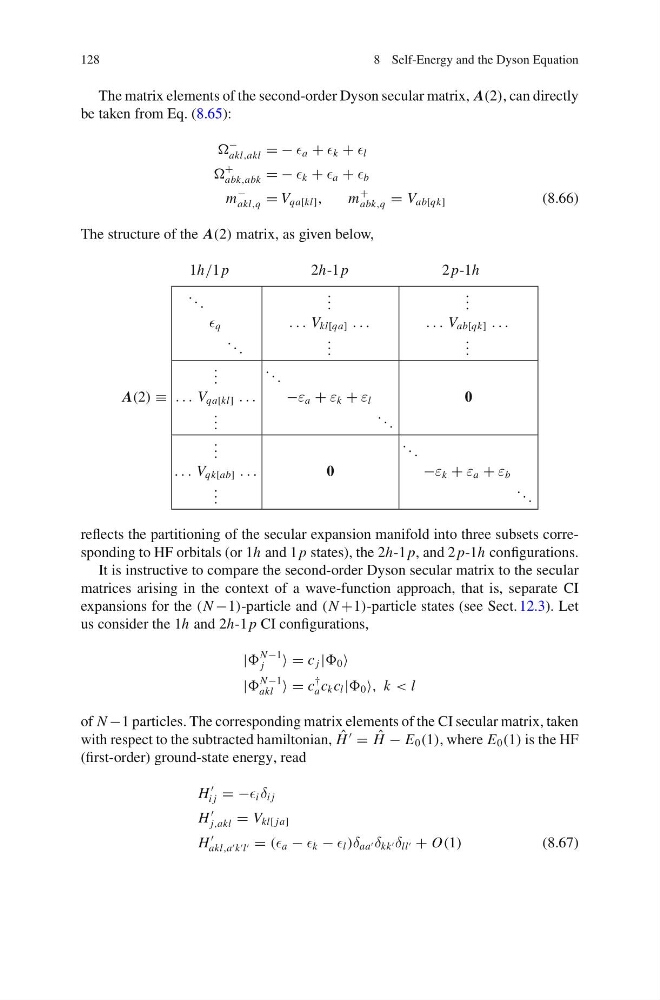
The structure of the A(2) matrix, as given below,
1h/1 p
2h-1 p
2 p-1h
A(2) ≡
. . .
q
. . .
. . .
. . . V kl[qa] . . .
. . .
. . .
. . . V ab[qk] . . .
. . .
. . .
. . . V qa[kl] . . .
. . .
. . .
−ε a + ε k + ε l
. . .
0
. . .
. . . V qk[ab] . . .
. . .
0
. . .
−ε k + ε a + ε b
. . .
reflects the partitioning of the secular expansion manifold into three subsets corresponding to HF orbitals (or 1h and 1 p states), the 2h-1 p, and 2 p-1h configurations.
It is instructive to compare the second-order Dyson secular matrix to the secular
matrices arising in the context of a wave-function approach, that is, separate CI
expansions for the (N −1)-particle and (N +1)-particle states (see Sect. 12.3). Let
us consider the 1h and 2h-1 p CI configurations,
|
N −1
j
= c j | 0
|
N −1
akl = c
†
a c k c l | 0 , k < l
of N −1 particles. The corresponding matrix elements of the CI secular matrix, taken
with respect to the subtracted hamiltonian, ˆ
H
= ˆ
H − E 0 (1), where E 0 (1) is the HF
(first-order) ground-state energy, read
H
i j = − i δ i j
H
j,akl = V kl[ ja]
H
akl,a k l = ( a − k − l )δ aa δ kk δ ll + O(1)
(8.67)
8 Self-Energy and the Dyson Equation
The matrix elements of the second-order Dyson secular matrix, A(2), can directly
be taken from Eq. (8.65):
−
akl,akl = − a + k + l
+
abk,abk = − k + a + b
m
−
akl,q = V qa[kl] ,
m
+
abk,q = V ab[qk]
(8.66)
The structure of the A(2) matrix, as given below,
1h/1 p
2h-1 p
2 p-1h
A(2) ≡
. . .
q
. . .
. . .
. . . V kl[qa] . . .
. . .
. . .
. . . V ab[qk] . . .
. . .
. . .
. . . V qa[kl] . . .
. . .
. . .
−ε a + ε k + ε l
. . .
0
. . .
. . . V qk[ab] . . .
. . .
0
. . .
−ε k + ε a + ε b
. . .
reflects the partitioning of the secular expansion manifold into three subsets corresponding to HF orbitals (or 1h and 1 p states), the 2h-1 p, and 2 p-1h configurations.
It is instructive to compare the second-order Dyson secular matrix to the secular
matrices arising in the context of a wave-function approach, that is, separate CI
expansions for the (N −1)-particle and (N +1)-particle states (see Sect. 12.3). Let
us consider the 1h and 2h-1 p CI configurations,
|
N −1
j
= c j | 0
|
N −1
akl = c
†
a c k c l | 0 , k < l
of N −1 particles. The corresponding matrix elements of the CI secular matrix, taken
with respect to the subtracted hamiltonian, ˆ
H
= ˆ
H − E 0 (1), where E 0 (1) is the HF
(first-order) ground-state energy, read
H
i j = − i δ i j
H
j,akl = V kl[ ja]
H
akl,a k l = ( a − k − l )δ aa δ kk δ ll + O(1)
(8.67)