

8.3 Solving the Dyson Equation
127
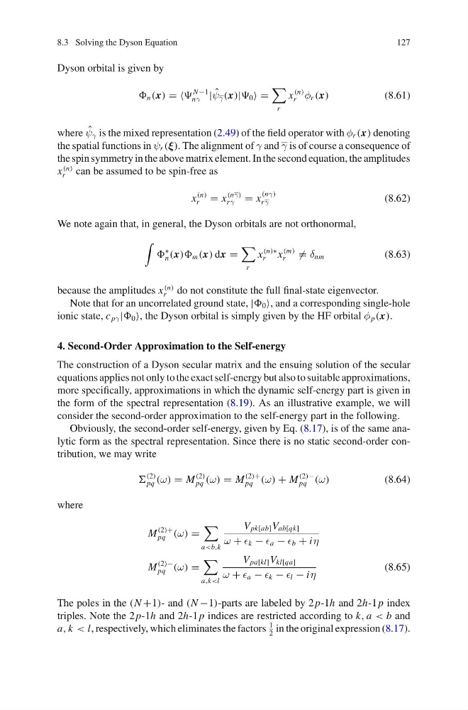
Dyson orbital is given by
n (x) = =
N −1
nγ | ˆ
ψ γ (x)| 0 =
r
x
(n)
r φ r (x)
(8.61)
where ˆ
ψ γ is the mixed representation (2.49) of the field operator with φ r (x) denoting
the spatial functions in ψ r (ξ). The alignment of γ and γ is of course a consequence of
the spin symmetry in the above matrix element. In the second equation, the amplitudes
x
(n)
r can be assumed to be spin-free as
x
(n)
r = x
(nγ)
r γ = x
(nγ)
r γ
(8.62)
We note again that, in general, the Dyson orbitals are not orthonormal,
∗
n (x)) m (x) dx =
r
x
(n)∗
r
x
(m)
r
= δ nm
(8.63)
because the amplitudes x
(n)
r do not constitute the full final-state eigenvector.
Note that for an uncorrelated ground state, | 0 , and a corresponding single-hole
ionic state, c pγ | 0 , the Dyson orbital is simply given by the HF orbital φ p (x).
4. Second-Order Approximation to the Self-energy
The construction of a Dyson secular matrix and the ensuing solution of the secular
equations applies not only to the exact self-energy but also to suitable approximations,
more specifically, approximations in which the dynamic self-energy part is given in
the form of the spectral representation (8.19). As an illustrative example, we will
consider the second-order approximation to the self-energy part in the following.
Obviously, the second-order self-energy, given by Eq. (8.17), is of the same analytic form as the spectral representation. Since there is no static second-order contribution, we may write
(2)
pq (ω) = M
(2)
pq (ω) = M
(2)+
pq (ω) + M
(2)−
pq (ω)
(8.64)
where
M
(2)+
pq (ω) =
a
ω + k − a − b + iη
M
(2)−
pq (ω) =
a,k
ω + a − k − l − iη
(8.65)
The poles in the (N +1)- and (N −1)-parts are labeled by 2 p-1h and 2h-1 p index
triples. Note the 2 p-1h and 2h-1 p indices are restricted according to k, a < b and
a, k < l, respectively, which eliminates the factors
1
2
in the original expression (8.17).
127
Dyson orbital is given by
n (x) = =
N −1
nγ | ˆ
ψ γ (x)| 0 =
r
x
(n)
r φ r (x)
(8.61)
where ˆ
ψ γ is the mixed representation (2.49) of the field operator with φ r (x) denoting
the spatial functions in ψ r (ξ). The alignment of γ and γ is of course a consequence of
the spin symmetry in the above matrix element. In the second equation, the amplitudes
x
(n)
r can be assumed to be spin-free as
x
(n)
r = x
(nγ)
r γ = x
(nγ)
r γ
(8.62)
We note again that, in general, the Dyson orbitals are not orthonormal,
∗
n (x)) m (x) dx =
r
x
(n)∗
r
x
(m)
r
= δ nm
(8.63)
because the amplitudes x
(n)
r do not constitute the full final-state eigenvector.
Note that for an uncorrelated ground state, | 0 , and a corresponding single-hole
ionic state, c pγ | 0 , the Dyson orbital is simply given by the HF orbital φ p (x).
4. Second-Order Approximation to the Self-energy
The construction of a Dyson secular matrix and the ensuing solution of the secular
equations applies not only to the exact self-energy but also to suitable approximations,
more specifically, approximations in which the dynamic self-energy part is given in
the form of the spectral representation (8.19). As an illustrative example, we will
consider the second-order approximation to the self-energy part in the following.
Obviously, the second-order self-energy, given by Eq. (8.17), is of the same analytic form as the spectral representation. Since there is no static second-order contribution, we may write
(2)
pq (ω) = M
(2)
pq (ω) = M
(2)+
pq (ω) + M
(2)−
pq (ω)
(8.64)
where
M
(2)+
pq (ω) =
a
ω + k − a − b + iη
M
(2)−
pq (ω) =
a,k
ω + a − k − l − iη
(8.65)
The poles in the (N +1)- and (N −1)-parts are labeled by 2 p-1h and 2h-1 p index
triples. Note the 2 p-1h and 2h-1 p indices are restricted according to k, a < b and
a, k < l, respectively, which eliminates the factors
1
2
in the original expression (8.17).