

8.2 Analytical Properties of the Self-Energy
121
(ω) = − + x Ex
†
+ O
1
ω
(8.29)
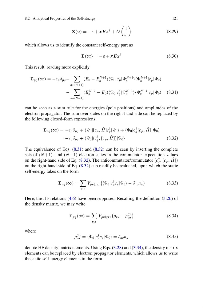
which allows us to identify the constant self-energy part as
(∞) = − + x Ex
†
(8.30)
This result, reading more explicitly
pq (∞) = − p δ pq −
n∈{N +1}
(E 0 − E
N +1
n
) 0 |c p |
N +1
n
N +1
n
|c
†
q | 0
−
n∈{N −1}
(E
N −1
n
− E 0 ) 0 |c
†
q |
N −1
n
N −1
n
|c p | 0 (8.31)
can be seen as a sum rule for the energies (pole positions) and amplitudes of the
electron propagator. The sum over states on the right-hand side can be replaced by
the following closed-form expressions:
pq (∞) = − p δ pq + + 0 |[c p , ˆ
H ]c
†
q | 0 + + 0 |c
†
q [c p , ˆ
H ]| 0
= − p δ pq + + 0 |{c
†
q , [c p , ˆ
H ]}| 0
(8.32)
The equivalence of Eqs. (8.31) and (8.32) can be seen by inserting the complete
sets of (N +1)- and (N −1)-electron states in the commutator expectation values
on the right-hand side of Eq. (8.32). The anticommutator/commutator {c
†
q , [c p , ˆ
H ]}
on the right-hand side of Eq. (8.32) can readily be evaluated, upon which the static
self-energy takes on the form
pq (∞) =
u,v
V pu[qv]
0 |c
†
u c v | 0 − δ uv n u
(8.33)
Here, the HF relations (4.6) have been supposed. Recalling the definition (3.26) of
the density matrix, we may write
pq (∞) =
u,v
V pu[qv]
ρ vu − ρ
(0)
vu
(8.34)
where
ρ
(0)
vu = = 0 |c
†
u c v | 0 = δ uv n u
(8.35)
denote HF density matrix elements. Using Eqs. (3.28) and (3.34), the density matrix
elements can be replaced by electron propagator elements, which allows us to write
the static self-energy elements in the form
121
(ω) = − + x Ex
†
+ O
1
ω
(8.29)
which allows us to identify the constant self-energy part as
(∞) = − + x Ex
†
(8.30)
This result, reading more explicitly
pq (∞) = − p δ pq −
n∈{N +1}
(E 0 − E
N +1
n
) 0 |c p |
N +1
n
N +1
n
|c
†
q | 0
−
n∈{N −1}
(E
N −1
n
− E 0 ) 0 |c
†
q |
N −1
n
N −1
n
|c p | 0 (8.31)
can be seen as a sum rule for the energies (pole positions) and amplitudes of the
electron propagator. The sum over states on the right-hand side can be replaced by
the following closed-form expressions:
pq (∞) = − p δ pq + + 0 |[c p , ˆ
H ]c
†
q | 0 + + 0 |c
†
q [c p , ˆ
H ]| 0
= − p δ pq + + 0 |{c
†
q , [c p , ˆ
H ]}| 0
(8.32)
The equivalence of Eqs. (8.31) and (8.32) can be seen by inserting the complete
sets of (N +1)- and (N −1)-electron states in the commutator expectation values
on the right-hand side of Eq. (8.32). The anticommutator/commutator {c
†
q , [c p , ˆ
H ]}
on the right-hand side of Eq. (8.32) can readily be evaluated, upon which the static
self-energy takes on the form
pq (∞) =
u,v
V pu[qv]
0 |c
†
u c v | 0 − δ uv n u
(8.33)
Here, the HF relations (4.6) have been supposed. Recalling the definition (3.26) of
the density matrix, we may write
pq (∞) =
u,v
V pu[qv]
ρ vu − ρ
(0)
vu
(8.34)
where
ρ
(0)
vu = = 0 |c
†
u c v | 0 = δ uv n u
(8.35)
denote HF density matrix elements. Using Eqs. (3.28) and (3.34), the density matrix
elements can be replaced by electron propagator elements, which allows us to write
the static self-energy elements in the form