

8.1 Diagrammatic Approach to the Self-Energy
117
2. Time-Ordered Diagrams for the Self-energy Part
(G1’) A Feynman (or Abrikosov) diagram of nth order gives rise to n! time-ordered
or Goldstone diagrams corresponding to the n! permutations of the two outer
vertices t, t
and n − 2 inner vertices t 1 , . . . , t n−2 . Draw an auxiliary line
(ω-line) from vertex t to vertex t
.
The other rules (G2)–(G4) apply in their original form. In particular, the overall phase
factor remains to be +1, which comes about as follows:
+1 ←
⎧
⎪ ⎪ ⎪ ⎪ ⎨
⎪ ⎪ ⎪ ⎪ ⎩
−i
from the definition of the propagator
(−i)
n
from the nth-order perturbation theory
i
n−1
from the N −1 cuts
i
2
from the two external free fermion lines
As an example, we will apply the Goldstone analysis to evaluate
(2)
pq (ω). The
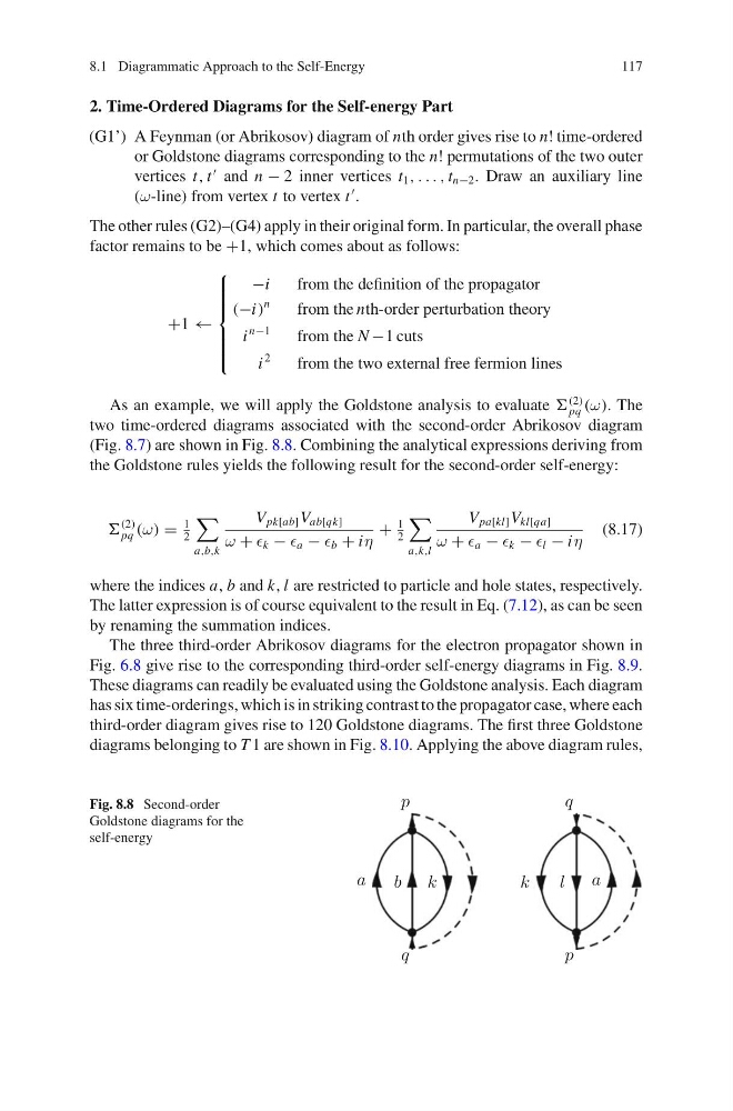
two time-ordered diagrams associated with the second-order Abrikosov diagram
(Fig. 8.7) are shown in Fig. 8.8. Combining the analytical expressions deriving from
the Goldstone rules yields the following result for the second-order self-energy:
(2)
pq (ω) =
1
2
a,b,k
V pk[ab] V ab[qk]
ω + k − a − b + iη
+
1
2
a,k,l
V pa[kl] V kl[qa]
ω + a − k − l − iη
(8.17)
where the indices a, b and k, l are restricted to particle and hole states, respectively.
The latter expression is of course equivalent to the result in Eq. (7.12), as can be seen
by renaming the summation indices.
The three third-order Abrikosov diagrams for the electron propagator shown in
Fig. 6.8 give rise to the corresponding third-order self-energy diagrams in Fig. 8.9.
These diagrams can readily be evaluated using the Goldstone analysis. Each diagram
has six time-orderings, which is in striking contrast to the propagator case, where each
third-order diagram gives rise to 120 Goldstone diagrams. The first three Goldstone
diagrams belonging to T 1 are shown in Fig. 8.10. Applying the above diagram rules,
Fig. 8.8 Second-order
Goldstone diagrams for the
self-energy
117
2. Time-Ordered Diagrams for the Self-energy Part
(G1’) A Feynman (or Abrikosov) diagram of nth order gives rise to n! time-ordered
or Goldstone diagrams corresponding to the n! permutations of the two outer
vertices t, t
and n − 2 inner vertices t 1 , . . . , t n−2 . Draw an auxiliary line
(ω-line) from vertex t to vertex t
.
The other rules (G2)–(G4) apply in their original form. In particular, the overall phase
factor remains to be +1, which comes about as follows:
+1 ←
⎧
⎪ ⎪ ⎪ ⎪ ⎨
⎪ ⎪ ⎪ ⎪ ⎩
−i
from the definition of the propagator
(−i)
n
from the nth-order perturbation theory
i
n−1
from the N −1 cuts
i
2
from the two external free fermion lines
As an example, we will apply the Goldstone analysis to evaluate
(2)
pq (ω). The
two time-ordered diagrams associated with the second-order Abrikosov diagram
(Fig. 8.7) are shown in Fig. 8.8. Combining the analytical expressions deriving from
the Goldstone rules yields the following result for the second-order self-energy:
(2)
pq (ω) =
1
2
a,b,k
V pk[ab] V ab[qk]
ω + k − a − b + iη
+
1
2
a,k,l
V pa[kl] V kl[qa]
ω + a − k − l − iη
(8.17)
where the indices a, b and k, l are restricted to particle and hole states, respectively.
The latter expression is of course equivalent to the result in Eq. (7.12), as can be seen
by renaming the summation indices.
The three third-order Abrikosov diagrams for the electron propagator shown in
Fig. 6.8 give rise to the corresponding third-order self-energy diagrams in Fig. 8.9.
These diagrams can readily be evaluated using the Goldstone analysis. Each diagram
has six time-orderings, which is in striking contrast to the propagator case, where each
third-order diagram gives rise to 120 Goldstone diagrams. The first three Goldstone
diagrams belonging to T 1 are shown in Fig. 8.10. Applying the above diagram rules,
Fig. 8.8 Second-order
Goldstone diagrams for the
self-energy