

116
8 Self-Energy and the Dyson Equation
(2)
pq (t, t
) =
1
2
r,u,v
V pr[uv] V uv[qr] G
0
u (t, t
)G
0
v (t, t
)G
0
r (t
, t)
(8.15)
In the energy representation (Eqs. (7.8), (7.9)) of the second-order electron propagator, the G
0 functions associated with the two outer free fermion lines factorize,
and
(2)
pq (ω) is obtained by simply discarding those G
0 -factors:
(2)
pq (ω) =
1
2
r,u,v
V pr[uv] V uv[qr]
dω 1
2π
dω 2
2π
G
0
u (ω 1 )G
0
v (ω 2 )G
0
r (ω 1 + ω 2 − ω)
(8.16)
The internal ω-integrations have been performed in Sect. 7.1 (cf. Eq. 7.10), and the
resulting explicit expression for
(2)
pq (ω) is given by Eq. (7.12). The rules presented in
Sect. 7.1 for evaluating diagrams in the energy representation can easily be adapted
to the case of the self-energy diagrams.
As discussed in Sect. 7.2, time-ordered or Goldstone diagrams can be used to
derive directly explicit ω-dependent expressions for the electron propagator diagrams. The same technique can be applied to the self-energy diagrams. In an nthorder self-energy diagram, there are n vertices. Hence, the number of time-orderings
is n! rather than (n + 2)!, which means a considerable reduction in comparison with
the case of the electron propagator. The original diagram rule (G1) must be modified
accordingly:
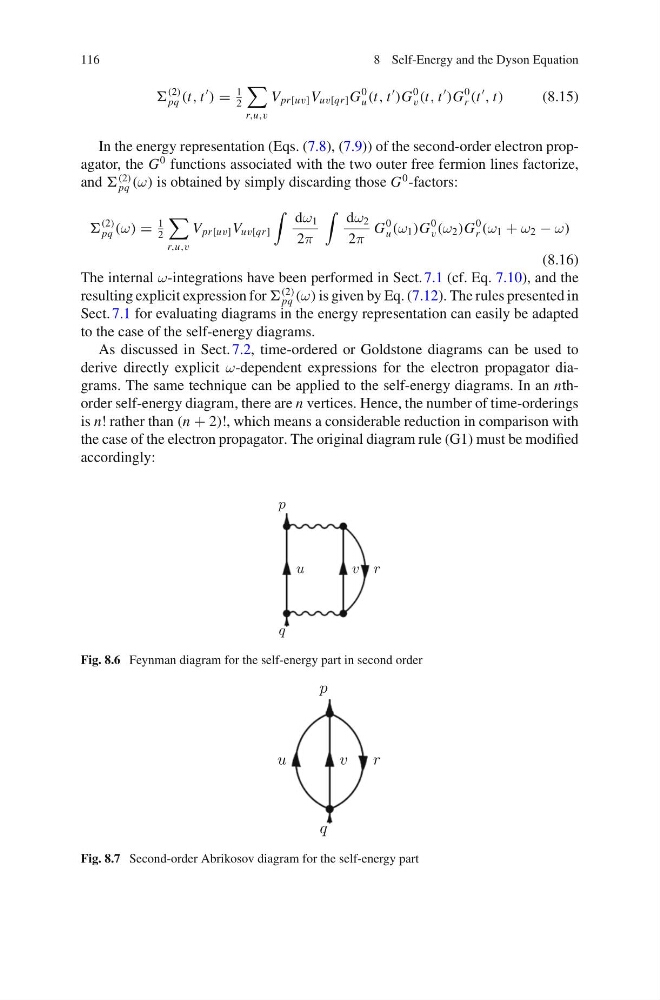
Fig. 8.6 Feynman diagram for the self-energy part in second order
Fig. 8.7 Second-order Abrikosov diagram for the self-energy part
8 Self-Energy and the Dyson Equation
(2)
pq (t, t
) =
1
2
r,u,v
V pr[uv] V uv[qr] G
0
u (t, t
)G
0
v (t, t
)G
0
r (t
, t)
(8.15)
In the energy representation (Eqs. (7.8), (7.9)) of the second-order electron propagator, the G
0 functions associated with the two outer free fermion lines factorize,
and
(2)
pq (ω) is obtained by simply discarding those G
0 -factors:
(2)
pq (ω) =
1
2
r,u,v
V pr[uv] V uv[qr]
dω 1
2π
dω 2
2π
G
0
u (ω 1 )G
0
v (ω 2 )G
0
r (ω 1 + ω 2 − ω)
(8.16)
The internal ω-integrations have been performed in Sect. 7.1 (cf. Eq. 7.10), and the
resulting explicit expression for
(2)
pq (ω) is given by Eq. (7.12). The rules presented in
Sect. 7.1 for evaluating diagrams in the energy representation can easily be adapted
to the case of the self-energy diagrams.
As discussed in Sect. 7.2, time-ordered or Goldstone diagrams can be used to
derive directly explicit ω-dependent expressions for the electron propagator diagrams. The same technique can be applied to the self-energy diagrams. In an nthorder self-energy diagram, there are n vertices. Hence, the number of time-orderings
is n! rather than (n + 2)!, which means a considerable reduction in comparison with
the case of the electron propagator. The original diagram rule (G1) must be modified
accordingly:
Fig. 8.6 Feynman diagram for the self-energy part in second order
Fig. 8.7 Second-order Abrikosov diagram for the self-energy part