

7.2 Performing the Inner Time Integrations
101
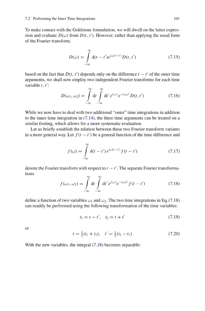
To make contact with the Goldstone formulation, we will dwell on the latter expression and evaluate D(ω) from D(t, t
). However, rather than applying the usual form
of the Fourier transform,
D(ω) =
∞
−∞
d(t − t
)e
iω(t−t
) D(t, t
)
(7.15)
based on the fact that D(t, t
) depends only on the difference t − t
of the outer time
arguments, we shall now employ two independent Fourier transforms for each time
variable t, t
:
D(ω 1 , ω 2 ) =
∞
−∞
dt
∞
−∞
dt
e
iω 1 t e
−iω 2 t
D(t, t
)
(7.16)
While we now have to deal with two additional “outer” time integrations in addition
to the inner time integration in (7.14), the three time arguments can be treated on a
similar footing, which allows for a more systematic evaluation.
Let us briefly establish the relation between these two Fourier transform variants
in a more general way. Let f (t − t
) be a general function of the time difference and
f (ω) =
∞
−∞
d(t − t
) e
iω(t−t
) f (t − t
)
(7.17)
denote the Fourier transform with respect to t − t
. The separate Fourier transformations
f (ω 1 , ω 2 ) =
∞
−∞
dt
∞
−∞
dt
e
iω 1 t e
−iω 2 t
f (t − t
)
(7.18)
define a function of two variables ω 1 and ω 2 . The two time integrations in Eq. (7.18)
can readily be performed using the following transformation of the time variables:
t 1 = t − t
, t 2 = t + t
(7.19)
or
t =
1
2
(t 1 + t 2 ), t
=
1
2
(t 2 − t 1 )
(7.20)
With the new variables, the integral (7.18) becomes separable:
101
To make contact with the Goldstone formulation, we will dwell on the latter expression and evaluate D(ω) from D(t, t
). However, rather than applying the usual form
of the Fourier transform,
D(ω) =
∞
−∞
d(t − t
)e
iω(t−t
) D(t, t
)
(7.15)
based on the fact that D(t, t
) depends only on the difference t − t
of the outer time
arguments, we shall now employ two independent Fourier transforms for each time
variable t, t
:
D(ω 1 , ω 2 ) =
∞
−∞
dt
∞
−∞
dt
e
iω 1 t e
−iω 2 t
D(t, t
)
(7.16)
While we now have to deal with two additional “outer” time integrations in addition
to the inner time integration in (7.14), the three time arguments can be treated on a
similar footing, which allows for a more systematic evaluation.
Let us briefly establish the relation between these two Fourier transform variants
in a more general way. Let f (t − t
) be a general function of the time difference and
f (ω) =
∞
−∞
d(t − t
) e
iω(t−t
) f (t − t
)
(7.17)
denote the Fourier transform with respect to t − t
. The separate Fourier transformations
f (ω 1 , ω 2 ) =
∞
−∞
dt
∞
−∞
dt
e
iω 1 t e
−iω 2 t
f (t − t
)
(7.18)
define a function of two variables ω 1 and ω 2 . The two time integrations in Eq. (7.18)
can readily be performed using the following transformation of the time variables:
t 1 = t − t
, t 2 = t + t
(7.19)
or
t =
1
2
(t 1 + t 2 ), t
=
1
2
(t 2 − t 1 )
(7.20)
With the new variables, the integral (7.18) becomes separable: