

102
7 Time-Ordered or Goldstone Diagrams
f (ω 1 , ω 2 ) =
1
2
∞
−∞
dt 1 e
i
ω 1 +ω 2
2
t 1 f (t 1 )
∞
−∞
dt 2 e
i
ω 1 −ω 2
2
t 2
= f (
ω 1 + ω 2
2
)
∞
−∞
dt 2
2
e
i
ω 1 −ω 2
2
t 2
= 2πδ(ω 1 − ω 2 ) f (ω 1 )
(7.21)
This establishes a simple relation between f (ω 1 , ω 2 ) and f (ω 1 ). The rule to obtain
f (ω) from f (ω 1 , ω 2 ) is to discard the factor 2πδ(ω 1 − ω 2 ), and replace both ω 1 and
ω 2 by ω.
The two-variable Fourier transform for the first-order diagram (7.14) takes on the
form
D(ω 1 , ω 2 ) = w pq
∞
−∞
dt
∞
−∞
dt
∞
−∞
dt 1 e
iω 1 t e
−iω 2 t
G
0
p (t, t 1 )G
0
q (t 1 , t
)
(7.22)
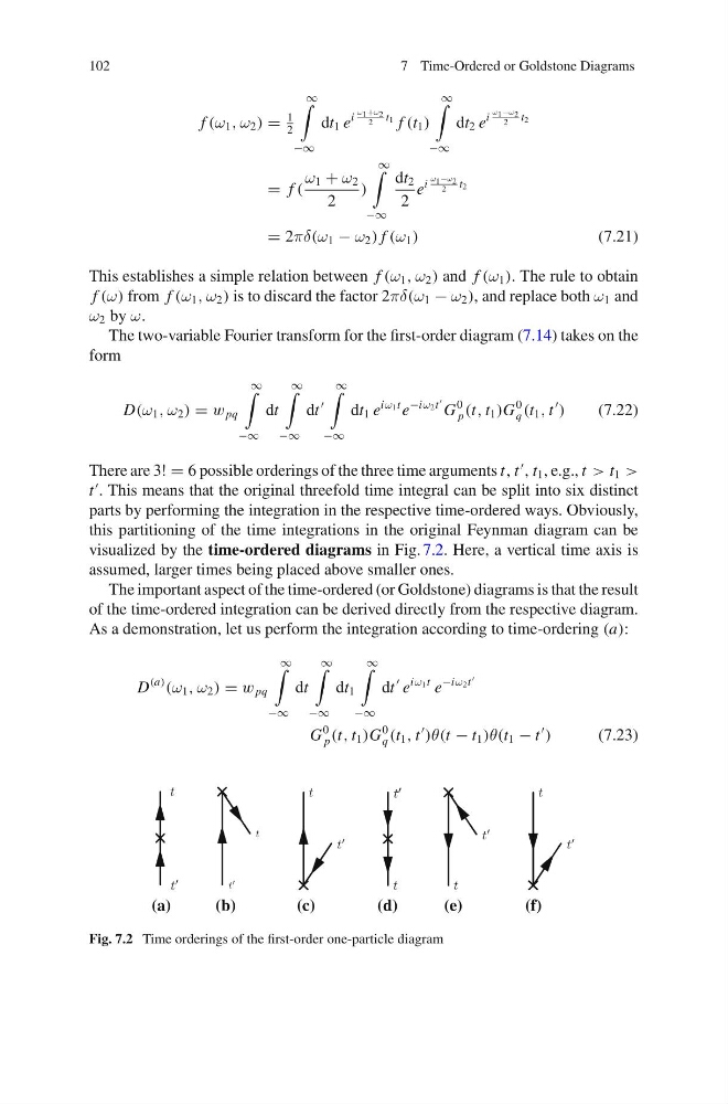
There are 3! = 6 possible orderings of the three time arguments t, t
, t 1 , e.g., t > t 1 >
t
. This means that the original threefold time integral can be split into six distinct
parts by performing the integration in the respective time-ordered ways. Obviously,
this partitioning of the time integrations in the original Feynman diagram can be
visualized by the time-ordered diagrams in Fig. 7.2. Here, a vertical time axis is
assumed, larger times being placed above smaller ones.
The important aspect of the time-ordered (or Goldstone) diagrams is that the result
of the time-ordered integration can be derived directly from the respective diagram.
As a demonstration, let us perform the integration according to time-ordering (a):
D
(a)
(ω 1 , ω 2 ) = w pq
∞
−∞
dt
∞
−∞
dt 1
∞
−∞
dt
e
iω 1 t e
−iω 2 t
G
0
p (t, t 1 )G
0
q (t 1 , t
)θ(t − t 1 )θ(t 1 − t
)
(7.23)
(a)
(b)
(c)
(d)
(e)
(f)
Fig. 7.2 Time orderings of the first-order one-particle diagram
7 Time-Ordered or Goldstone Diagrams
f (ω 1 , ω 2 ) =
1
2
∞
−∞
dt 1 e
i
ω 1 +ω 2
2
t 1 f (t 1 )
∞
−∞
dt 2 e
i
ω 1 −ω 2
2
t 2
= f (
ω 1 + ω 2
2
)
∞
−∞
dt 2
2
e
i
ω 1 −ω 2
2
t 2
= 2πδ(ω 1 − ω 2 ) f (ω 1 )
(7.21)
This establishes a simple relation between f (ω 1 , ω 2 ) and f (ω 1 ). The rule to obtain
f (ω) from f (ω 1 , ω 2 ) is to discard the factor 2πδ(ω 1 − ω 2 ), and replace both ω 1 and
ω 2 by ω.
The two-variable Fourier transform for the first-order diagram (7.14) takes on the
form
D(ω 1 , ω 2 ) = w pq
∞
−∞
dt
∞
−∞
dt
∞
−∞
dt 1 e
iω 1 t e
−iω 2 t
G
0
p (t, t 1 )G
0
q (t 1 , t
)
(7.22)
There are 3! = 6 possible orderings of the three time arguments t, t
, t 1 , e.g., t > t 1 >
t
. This means that the original threefold time integral can be split into six distinct
parts by performing the integration in the respective time-ordered ways. Obviously,
this partitioning of the time integrations in the original Feynman diagram can be
visualized by the time-ordered diagrams in Fig. 7.2. Here, a vertical time axis is
assumed, larger times being placed above smaller ones.
The important aspect of the time-ordered (or Goldstone) diagrams is that the result
of the time-ordered integration can be derived directly from the respective diagram.
As a demonstration, let us perform the integration according to time-ordering (a):
D
(a)
(ω 1 , ω 2 ) = w pq
∞
−∞
dt
∞
−∞
dt 1
∞
−∞
dt
e
iω 1 t e
−iω 2 t
G
0
p (t, t 1 )G
0
q (t 1 , t
)θ(t − t 1 )θ(t 1 − t
)
(7.23)
(a)
(b)
(c)
(d)
(e)
(f)
Fig. 7.2 Time orderings of the first-order one-particle diagram