

7.1 Energy Representation of Diagrams
99
G
0
v (ω 2 )G
0
r (ω 1 + ω 2 − ω) =n v n r (ω 2 − v + iη)
−1
(ω 1 + ω 2 − ω − r + iη)
−1
+ n v n r (· · · − iη)
−1
(· · · − iη)
−1
+ n v n r (· · · + iη)
−1
(· · · − iη)
−1
+ n v n r (· · · − iη)
−1
(· · · + iη)
−1
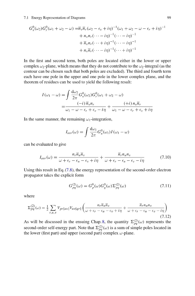
In the first and second term, both poles are located either in the lower or upper
complex ω 2 -plane, which means that they do not contribute to the ω 2 -integral (as the
contour can be chosen such that both poles are excluded). The third and fourth term
each have one pole in the upper and one pole in the lower complex plane, and the
theorem of residues can be used to yield the following result:
I (ω 1 − ω) =
dω 2
2π
G
0
v (ω 2 )G
0
r (ω 1 + ω 2 − ω)
=
(−i) n v n r
ω 1 − ω − r + v − iη
+
(+i) n v n r
ω 1 − ω − r + v + iη
In the same manner, the remaining ω 1 -integration,
I uvr (ω) =
dω 1
2π
G
0
u (ω 1 )I (ω 1 − ω)
can be evaluated to give
I uvr (ω) =
n r n u n v
ω + r − u − v + iη
+
n r n u n v
ω + r − u − v − iη
(7.10)
Using this result in Eq. (7.8), the energy representation of the second-order electron
propagator takes the explicit form
G
(2)
pq (ω) = G
0
p (ω)G
0
q (ω))
(2)
pq (ω)
(7.11)
where
(2)
pq (ω) = 1
2
r,u,v
V pr[uv] V uv[qr]
n r n u n v
ω + r − u − v + iη
+
n r n u n v
ω + r − u − v − iη
(7.12)
As will be discussed in the ensuing Chap. 8, the quantity
(2)
pq (ω) represents the
second-order self-energy part. Note that
(2)
pq (ω) is a sum of simple poles located in
the lower (first part) and upper (second part) complex ω-plane.
99
G
0
v (ω 2 )G
0
r (ω 1 + ω 2 − ω) =n v n r (ω 2 − v + iη)
−1
(ω 1 + ω 2 − ω − r + iη)
−1
+ n v n r (· · · − iη)
−1
(· · · − iη)
−1
+ n v n r (· · · + iη)
−1
(· · · − iη)
−1
+ n v n r (· · · − iη)
−1
(· · · + iη)
−1
In the first and second term, both poles are located either in the lower or upper
complex ω 2 -plane, which means that they do not contribute to the ω 2 -integral (as the
contour can be chosen such that both poles are excluded). The third and fourth term
each have one pole in the upper and one pole in the lower complex plane, and the
theorem of residues can be used to yield the following result:
I (ω 1 − ω) =
dω 2
2π
G
0
v (ω 2 )G
0
r (ω 1 + ω 2 − ω)
=
(−i) n v n r
ω 1 − ω − r + v − iη
+
(+i) n v n r
ω 1 − ω − r + v + iη
In the same manner, the remaining ω 1 -integration,
I uvr (ω) =
dω 1
2π
G
0
u (ω 1 )I (ω 1 − ω)
can be evaluated to give
I uvr (ω) =
n r n u n v
ω + r − u − v + iη
+
n r n u n v
ω + r − u − v − iη
(7.10)
Using this result in Eq. (7.8), the energy representation of the second-order electron
propagator takes the explicit form
G
(2)
pq (ω) = G
0
p (ω)G
0
q (ω))
(2)
pq (ω)
(7.11)
where
(2)
pq (ω) = 1
2
r,u,v
V pr[uv] V uv[qr]
n r n u n v
ω + r − u − v + iη
+
n r n u n v
ω + r − u − v − iη
(7.12)
As will be discussed in the ensuing Chap. 8, the quantity
(2)
pq (ω) represents the
second-order self-energy part. Note that
(2)
pq (ω) is a sum of simple poles located in
the lower (first part) and upper (second part) complex ω-plane.