

98
7 Time-Ordered or Goldstone Diagrams
The procedure of replacing the time by ω-integrations can readily be generalized
to arbitrary nth-order diagrams. This leads to the following modifications in the original diagram rules.
Feynman/Abrikosov Diagrams in Energy Representation
1. Assign ω-variables to the 2n + 1 free fermion lines and use the corresponding
energy representations, G
0
r (ω). Chose the (global) energy variable ω for the first
(incoming) outer free fermion line (G
0
q (ω)), and inner ω-variables, ω 1 , ω 2 , . . . ,
for the other free fermion lines.
2. Use energy conservation at each of the n inner vertices: ω i + ω i = ω o + ω o ,
where i, i
(o, o
) refer to incoming (outgoing) free fermion lines at a given vertex. These n conditions ensure that there are n independent inner ω-variables,
ω 1 , . . . , ω n , and the second (outgoing) outer free fermion line becomes G
0
p (ω).
3. Perform the n inner ω-integrations
dω 1
2π
. . .
dω n
2π
.
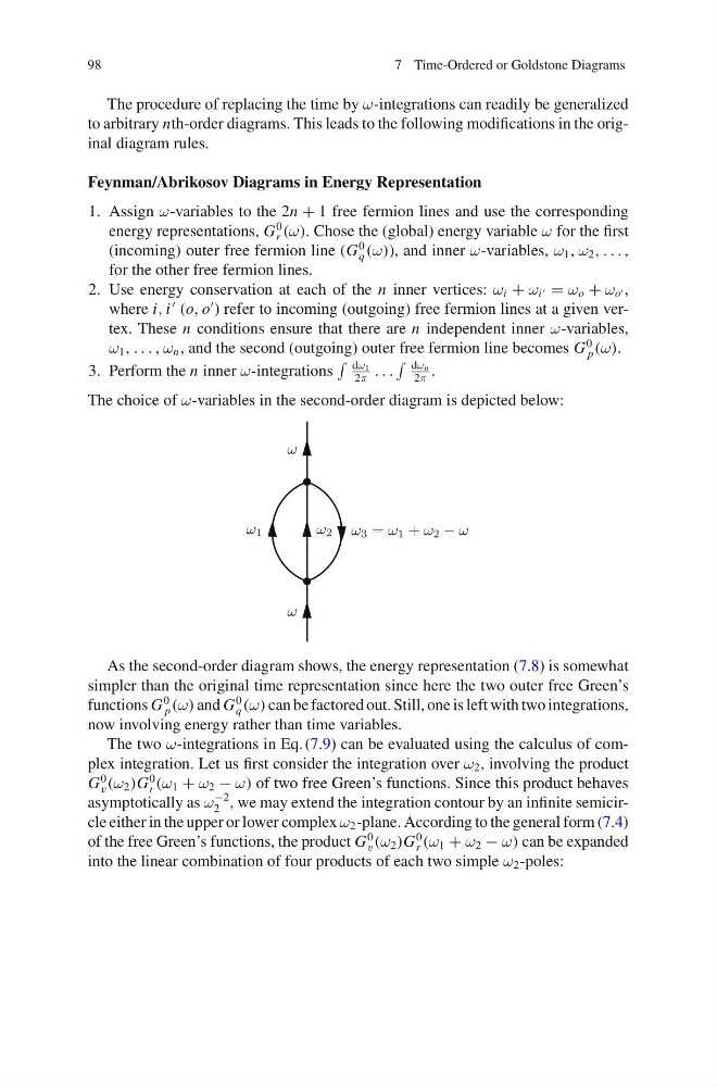
The choice of ω-variables in the second-order diagram is depicted below:
ω
ω 1
ω 2 ω 3 = ω 1 + ω 2 − ω
ω
As the second-order diagram shows, the energy representation (7.8) is somewhat
simpler than the original time representation since here the two outer free Green’s
functions G
0
p (ω) and G
0
q (ω) can be factored out. Still, one is left with two integrations,
now involving energy rather than time variables.
The two ω-integrations in Eq. (7.9) can be evaluated using the calculus of complex integration. Let us first consider the integration over ω 2 , involving the product
G
0
v (ω 2 )G
0
r (ω 1 + ω 2 − ω) of two free Green’s functions. Since this product behaves
asymptotically as ω
−2
2 , we may extend the integration contour by an infinite semicircle either in the upper or lower complex ω 2 -plane. According to the general form (7.4)
of the free Green’s functions, the product G
0
v (ω 2 )G
0
r (ω 1 + ω 2 − ω) can be expanded
into the linear combination of four products of each two simple ω 2 -poles:
7 Time-Ordered or Goldstone Diagrams
The procedure of replacing the time by ω-integrations can readily be generalized
to arbitrary nth-order diagrams. This leads to the following modifications in the original diagram rules.
Feynman/Abrikosov Diagrams in Energy Representation
1. Assign ω-variables to the 2n + 1 free fermion lines and use the corresponding
energy representations, G
0
r (ω). Chose the (global) energy variable ω for the first
(incoming) outer free fermion line (G
0
q (ω)), and inner ω-variables, ω 1 , ω 2 , . . . ,
for the other free fermion lines.
2. Use energy conservation at each of the n inner vertices: ω i + ω i = ω o + ω o ,
where i, i
(o, o
) refer to incoming (outgoing) free fermion lines at a given vertex. These n conditions ensure that there are n independent inner ω-variables,
ω 1 , . . . , ω n , and the second (outgoing) outer free fermion line becomes G
0
p (ω).
3. Perform the n inner ω-integrations
dω 1
2π
. . .
dω n
2π
.
The choice of ω-variables in the second-order diagram is depicted below:
ω
ω 1
ω 2 ω 3 = ω 1 + ω 2 − ω
ω
As the second-order diagram shows, the energy representation (7.8) is somewhat
simpler than the original time representation since here the two outer free Green’s
functions G
0
p (ω) and G
0
q (ω) can be factored out. Still, one is left with two integrations,
now involving energy rather than time variables.
The two ω-integrations in Eq. (7.9) can be evaluated using the calculus of complex integration. Let us first consider the integration over ω 2 , involving the product
G
0
v (ω 2 )G
0
r (ω 1 + ω 2 − ω) of two free Green’s functions. Since this product behaves
asymptotically as ω
−2
2 , we may extend the integration contour by an infinite semicircle either in the upper or lower complex ω 2 -plane. According to the general form (7.4)
of the free Green’s functions, the product G
0
v (ω 2 )G
0
r (ω 1 + ω 2 − ω) can be expanded
into the linear combination of four products of each two simple ω 2 -poles: