

4.2.2 Polarizabilities of X 2 –Y Complexes
Consider in this Section the complexes X 2 –Y when the atom Y has the spherical
symmetry. For another case the calculations are carried out the same way. The
Cartesian coordinate system is introduced following to Fig. 3.1. Then, for considered complex the induction contributions to Da
AB
ab ðRÞ up to terms *R
−6 inclusive
take the form [45]
a
ind
ab ¼ a
A
ac T cd a
B
db þ a
B
ac T cd a
A
db þ
1
15
a
A
ac T cdeu E
B
b;deu þ
1
15
E
B
a;cde T cdeu a
A
ub
À
1
9
B
A
ab;cd T cdeu H
B
eu þ a
A
ac T cd a
B
de T eu a
A
ub þ a
B
ac T cd a
A
de T eu a
B
ub :
ð4:2:7Þ
Dispersion contribution into Da
AB
ab ðRÞ following the results of Sect. 4.1.2 with
accuracy up to the leading term *R
−6 comes on (4.1.8). For this case the tensors
C gc ¼
1
6 C
0
6 d gc ; D xx ¼ D yy ¼
1
6 C
0
6 À C
2
6
À
Á
and D zz ¼
1
6 C
0
6 þ 2C
2
6
À
Á
are related to the
isotropic dispersion coefficient C
0
6 and the anisotropic dispersion coefficients C
2
6 .
The exchange contributions to the interaction polarizabilities are described by
Eq. (4.1.12) where the parameters B 1 and B 2 are the functions of the angle h and
can be written as [59]
B i ¼ B
ð0Þ
i þ B
ð2Þ
i P 2 ðcos hÞ þ B
ð4Þ
i P 4 ðcos hÞ
ð 4:2:8Þ
where P k ðcos hÞ is the Legendre polynomial and B
ðkÞ
i are the fitting parameters. The
full analytical expressions for the interaction polarizability of the complex X–Y 2 is
quite cumbersome and can be found in the work [59].
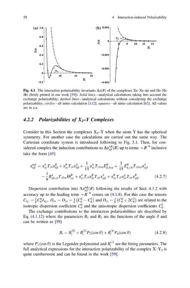
Fig. 4.1 The interaction polarizability invariants DaðRÞ of the complexes Xe–Xe (a) and He–He
(b) (firstly printed in our work [59]). Solid lines—analytical calculations taking into account the
exchange polarizability; dashed lines—analytical calculations without considering the exchange
polarizability; circles—ab initio calculation [112]; squares—ab initio calculation [62]. All values
are in a.u
58
4 Interaction-induced Polarizability
Consider in this Section the complexes X 2 –Y when the atom Y has the spherical
symmetry. For another case the calculations are carried out the same way. The
Cartesian coordinate system is introduced following to Fig. 3.1. Then, for considered complex the induction contributions to Da
AB
ab ðRÞ up to terms *R
−6 inclusive
take the form [45]
a
ind
ab ¼ a
A
ac T cd a
B
db þ a
B
ac T cd a
A
db þ
1
15
a
A
ac T cdeu E
B
b;deu þ
1
15
E
B
a;cde T cdeu a
A
ub
À
1
9
B
A
ab;cd T cdeu H
B
eu þ a
A
ac T cd a
B
de T eu a
A
ub þ a
B
ac T cd a
A
de T eu a
B
ub :
ð4:2:7Þ
Dispersion contribution into Da
AB
ab ðRÞ following the results of Sect. 4.1.2 with
accuracy up to the leading term *R
−6 comes on (4.1.8). For this case the tensors
C gc ¼
1
6 C
0
6 d gc ; D xx ¼ D yy ¼
1
6 C
0
6 À C
2
6
À
Á
and D zz ¼
1
6 C
0
6 þ 2C
2
6
À
Á
are related to the
isotropic dispersion coefficient C
0
6 and the anisotropic dispersion coefficients C
2
6 .
The exchange contributions to the interaction polarizabilities are described by
Eq. (4.1.12) where the parameters B 1 and B 2 are the functions of the angle h and
can be written as [59]
B i ¼ B
ð0Þ
i þ B
ð2Þ
i P 2 ðcos hÞ þ B
ð4Þ
i P 4 ðcos hÞ
ð 4:2:8Þ
where P k ðcos hÞ is the Legendre polynomial and B
ðkÞ
i are the fitting parameters. The
full analytical expressions for the interaction polarizability of the complex X–Y 2 is
quite cumbersome and can be found in the work [59].
Fig. 4.1 The interaction polarizability invariants DaðRÞ of the complexes Xe–Xe (a) and He–He
(b) (firstly printed in our work [59]). Solid lines—analytical calculations taking into account the
exchange polarizability; dashed lines—analytical calculations without considering the exchange
polarizability; circles—ab initio calculation [112]; squares—ab initio calculation [62]. All values
are in a.u
58
4 Interaction-induced Polarizability