

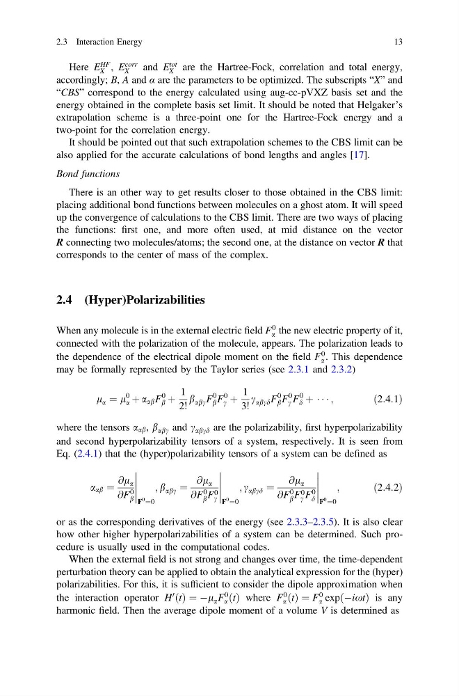
Here E
HF
X , E
corr
X
and E
tot
X are the Hartree-Fock, correlation and total energy,
accordingly; B, A and α are the parameters to be optimized. The subscripts “X” and
“CBS” correspond to the energy calculated using aug-cc-pVXZ basis set and the
energy obtained in the complete basis set limit. It should be noted that Helgaker’s
extrapolation scheme is a three-point one for the Hartree-Fock energy and a
two-point for the correlation energy.
It should be pointed out that such extrapolation schemes to the CBS limit can be
also applied for the accurate calculations of bond lengths and angles [17].
Bond functions
There is an other way to get results closer to those obtained in the CBS limit:
placing additional bond functions between molecules on a ghost atom. It will speed
up the convergence of calculations to the CBS limit. There are two ways of placing
the functions: first one, and more often used, at mid distance on the vector
R connecting two molecules/atoms; the second one, at the distance on vector R that
corresponds to the center of mass of the complex.
2.4 (Hyper)Polarizabilities
When any molecule is in the external electric field F
0
a the new electric property of it,
connected with the polarization of the molecule, appears. The polarization leads to
the dependence of the electrical dipole moment on the field F
0
a . This dependence
may be formally represented by the Taylor series (see 2.3.1 and 2.3.2)
l a ¼ l
0
a þ a ab F
0
b þ
1
2!
b abc F
0
b F
0
c þ
1
3!
c abcd F
0
b F
0
c F
0
d þ Á Á Á ;
ð2:4:1Þ
where the tensors a ab , b abc and c abcd are the polarizability, first hyperpolarizability
and second hyperpolarizability tensors of a system, respectively. It is seen from
Eq. (2.4.1) that the (hyper)polarizability tensors of a system can be defined as
a ab ¼
@l a
@F
0
b
F
0 ¼0
; b abc ¼
@l a
@F
0
b F 0
c
F
0 ¼0
; c abcd ¼
@l a
@F
0
b F 0
c F
0
d
F
0 ¼0
;
ð2:4:2Þ
or as the corresponding derivatives of the energy (see 2.3.3–2.3.5). It is also clear
how other higher hyperpolarizabilities of a system can be determined. Such procedure is usually used in the computational codes.
When the external field is not strong and changes over time, the time-dependent
perturbation theory can be applied to obtain the analytical expression for the (hyper)
polarizabilities. For this, it is sufficient to consider the dipole approximation when
the interaction operator H
0
ðtÞ ¼ Àl a F
0
a ðtÞ where F
0
a ðtÞ ¼ F
0
a expðÀixtÞ is any
harmonic field. Then the average dipole moment of a volume V is determined as
2.3 Interaction Energy
13
HF
X , E
corr
X
and E
tot
X are the Hartree-Fock, correlation and total energy,
accordingly; B, A and α are the parameters to be optimized. The subscripts “X” and
“CBS” correspond to the energy calculated using aug-cc-pVXZ basis set and the
energy obtained in the complete basis set limit. It should be noted that Helgaker’s
extrapolation scheme is a three-point one for the Hartree-Fock energy and a
two-point for the correlation energy.
It should be pointed out that such extrapolation schemes to the CBS limit can be
also applied for the accurate calculations of bond lengths and angles [17].
Bond functions
There is an other way to get results closer to those obtained in the CBS limit:
placing additional bond functions between molecules on a ghost atom. It will speed
up the convergence of calculations to the CBS limit. There are two ways of placing
the functions: first one, and more often used, at mid distance on the vector
R connecting two molecules/atoms; the second one, at the distance on vector R that
corresponds to the center of mass of the complex.
2.4 (Hyper)Polarizabilities
When any molecule is in the external electric field F
0
a the new electric property of it,
connected with the polarization of the molecule, appears. The polarization leads to
the dependence of the electrical dipole moment on the field F
0
a . This dependence
may be formally represented by the Taylor series (see 2.3.1 and 2.3.2)
l a ¼ l
0
a þ a ab F
0
b þ
1
2!
b abc F
0
b F
0
c þ
1
3!
c abcd F
0
b F
0
c F
0
d þ Á Á Á ;
ð2:4:1Þ
where the tensors a ab , b abc and c abcd are the polarizability, first hyperpolarizability
and second hyperpolarizability tensors of a system, respectively. It is seen from
Eq. (2.4.1) that the (hyper)polarizability tensors of a system can be defined as
a ab ¼
@l a
@F
0
b
F
0 ¼0
; b abc ¼
@l a
@F
0
b F 0
c
F
0 ¼0
; c abcd ¼
@l a
@F
0
b F 0
c F
0
d
F
0 ¼0
;
ð2:4:2Þ
or as the corresponding derivatives of the energy (see 2.3.3–2.3.5). It is also clear
how other higher hyperpolarizabilities of a system can be determined. Such procedure is usually used in the computational codes.
When the external field is not strong and changes over time, the time-dependent
perturbation theory can be applied to obtain the analytical expression for the (hyper)
polarizabilities. For this, it is sufficient to consider the dipole approximation when
the interaction operator H
0
ðtÞ ¼ Àl a F
0
a ðtÞ where F
0
a ðtÞ ¼ F
0
a expðÀixtÞ is any
harmonic field. Then the average dipole moment of a volume V is determined as
2.3 Interaction Energy
13