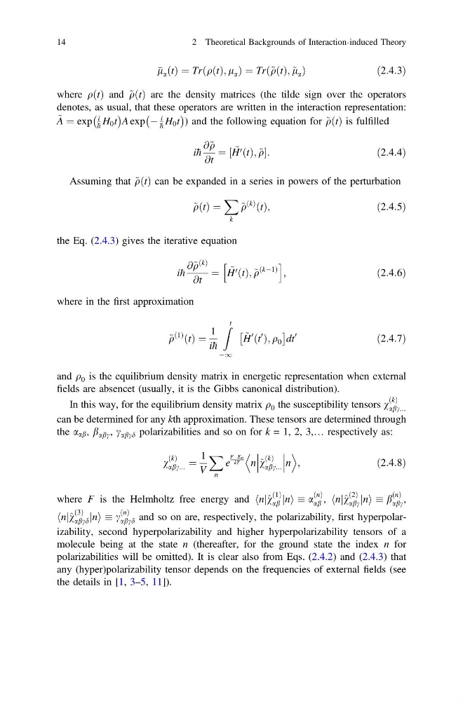
l a ðtÞ ¼ TrðqðtÞ; l a Þ ¼ Trð~ qðtÞ; ~
l a Þ
ð 2:4:3Þ
where qðtÞ and ~
qðtÞ are the density matrices (the tilde sign over the operators
denotes, as usual, that these operators are written in the interaction representation:
~
A ¼ exp
i
h H 0 t
À
Á
A exp À
i
h H 0 t
À
Á
) and the following equation for ~
qðtÞ is fulfilled
i h
@~ q
@t
¼ ½ ~
H 0 ðtÞ; ~
qŠ:
ð2:4:4Þ
Assuming that ~
qðtÞ can be expanded in a series in powers of the perturbation
~
qðtÞ ¼
X
k
~
q
ðkÞ
ðtÞ;
ð2:4:5Þ
the Eq. (2.4.3) gives the iterative equation
i h
@~ q
ðkÞ
@t
¼ ~
H 0 ðtÞ; ~
q
ðkÀ1Þ
h
i
;
ð2:4:6Þ
where in the first approximation
~
q
ð1Þ
ðtÞ ¼
1
i h
Z t
À1
~
H
0
ðt
0
Þ; q 0
Â
Ã
dt
0
ð2:4:7Þ
and q 0 is the equilibrium density matrix in energetic representation when external
fields are absencet (usually, it is the Gibbs canonical distribution).
In this way, for the equilibrium density matrix q 0 the susceptibility tensors v
ðkÞ
abc...
can be determined for any kth approximation. These tensors are determined through
the a ab , b abc , c abcd polarizabilities and so on for k = 1, 2, 3,… respectively as:
v
ðkÞ
abc... ¼
1
V
X
n
e
FÀEn
kT
n ^ v
ðkÞ
abc...
n
D
E
;
ð2:4:8Þ
where F is the Helmholtz free energy and n
h j^ v
ð1Þ
ab n
j i a
ðnÞ
ab , n
h j^ v
ð2Þ
abc n
j i b
ðnÞ
abc ,
n
h j^ v
ð3Þ
abcd n
j i c
ðnÞ
abcd and so on are, respectively, the polarizability, first hyperpolarizability, second hyperpolarizability and higher hyperpolarizability tensors of a
molecule being at the state n (thereafter, for the ground state the index n for
polarizabilities will be omitted). It is clear also from Eqs. (2.4.2) and (2.4.3) that
any (hyper)polarizability tensor depends on the frequencies of external fields (see
the details in [1, 3–5, 11]).
14
2 Theoretical Backgrounds of Interaction-induced Theory