

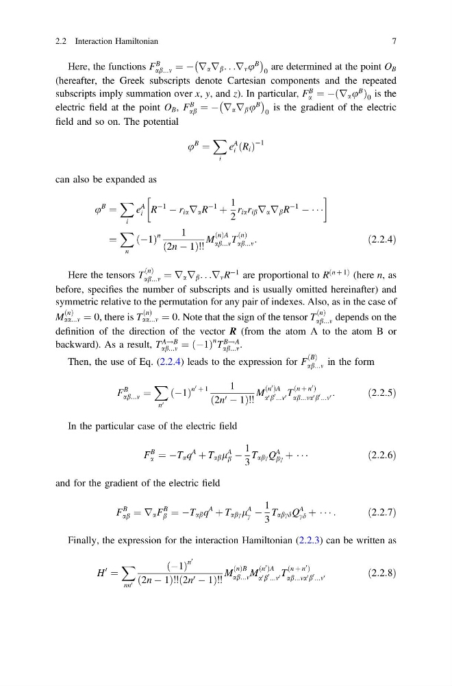
Here, the functions F
B
ab...m ¼ À r a r b . . .r m u
B
À
Á
0
are determined at the point O B
(hereafter, the Greek subscripts denote Cartesian components and the repeated
subscripts imply summation over x, y, and z). In particular, F
B
a ¼ À r a u
B
ð
Þ 0 is the
electric field at the point O B , F
B
ab ¼ À r a r b u
B
À
Á
0
is the gradient of the electric
field and so on. The potential
u
B
¼
X
i
e
A
i R i
ð Þ
À1
can also be expanded as
u
B
¼
X
i
e
A
i R
À1
À r ia r a R
À1
þ
1
2
r ia r ib r a r b R
À1
À Á Á Á
!
¼
X
n
ðÀ1Þ
n
1
ð2n À 1Þ!!
M
ðnÞA
ab...m T
ðnÞ
ab...m :
ð2:2:4Þ
Here the tensors T
ðnÞ
ab...m ¼ r a r b . . .r m R
À1 are proportional to R
ðn þ 1Þ (here n, as
before, specifies the number of subscripts and is usually omitted hereinafter) and
symmetric relative to the permutation for any pair of indexes. Also, as in the case of
M
ðnÞ
aa...m ¼ 0, there is T
ðnÞ
aa...m ¼ 0. Note that the sign of the tensor T
ðnÞ
ab...m depends on the
definition of the direction of the vector R (from the atom A to the atom B or
backward). As a result, T
A!B
ab...m ¼ ðÀ1Þ
n T
B!A
ab...m .
Then, the use of Eq. (2.2.4) leads to the expression for F
ðBÞ
ab...m in the form
F
B
ab...m ¼
X
n 0
ðÀ1Þ
n
0 þ 1
1
ð2n 0 À 1Þ!!
M
ðn
0 ÞA
a 0 b
0 ...m 0 T
ðn þ n
0 Þ
ab...ma 0 b
0 ...m 0 :
ð2:2:5Þ
In the particular case of the electric field
F
B
a ¼ ÀT a q
A
þ T ab l
A
b À
1
3
T abc Q
A
bc þ Á Á Á
ð2:2:6Þ
and for the gradient of the electric field
F
B
ab ¼ r a F
B
b ¼ ÀT ab q
A
þ T abc l
A
c À
1
3
T abcd Q
A
cd þ Á Á Á :
ð2:2:7Þ
Finally, the expression for the interaction Hamiltonian (2.2.3) can be written as
H
0
¼
X
nn 0
ðÀ1Þ
n
0
ð2n À 1Þ!!ð2n 0 À 1Þ!!
M
ðnÞB
ab...m M
ðn
0 ÞA
a 0 b
0 ...m 0 T
ðn þ n
0 Þ
ab...ma 0 b
0 ...m 0
ð2:2:8Þ
2.2 Interaction Hamiltonian
7
B
ab...m ¼ À r a r b . . .r m u
B
À
Á
0
are determined at the point O B
(hereafter, the Greek subscripts denote Cartesian components and the repeated
subscripts imply summation over x, y, and z). In particular, F
B
a ¼ À r a u
B
ð
Þ 0 is the
electric field at the point O B , F
B
ab ¼ À r a r b u
B
À
Á
0
is the gradient of the electric
field and so on. The potential
u
B
¼
X
i
e
A
i R i
ð Þ
À1
can also be expanded as
u
B
¼
X
i
e
A
i R
À1
À r ia r a R
À1
þ
1
2
r ia r ib r a r b R
À1
À Á Á Á
!
¼
X
n
ðÀ1Þ
n
1
ð2n À 1Þ!!
M
ðnÞA
ab...m T
ðnÞ
ab...m :
ð2:2:4Þ
Here the tensors T
ðnÞ
ab...m ¼ r a r b . . .r m R
À1 are proportional to R
ðn þ 1Þ (here n, as
before, specifies the number of subscripts and is usually omitted hereinafter) and
symmetric relative to the permutation for any pair of indexes. Also, as in the case of
M
ðnÞ
aa...m ¼ 0, there is T
ðnÞ
aa...m ¼ 0. Note that the sign of the tensor T
ðnÞ
ab...m depends on the
definition of the direction of the vector R (from the atom A to the atom B or
backward). As a result, T
A!B
ab...m ¼ ðÀ1Þ
n T
B!A
ab...m .
Then, the use of Eq. (2.2.4) leads to the expression for F
ðBÞ
ab...m in the form
F
B
ab...m ¼
X
n 0
ðÀ1Þ
n
0 þ 1
1
ð2n 0 À 1Þ!!
M
ðn
0 ÞA
a 0 b
0 ...m 0 T
ðn þ n
0 Þ
ab...ma 0 b
0 ...m 0 :
ð2:2:5Þ
In the particular case of the electric field
F
B
a ¼ ÀT a q
A
þ T ab l
A
b À
1
3
T abc Q
A
bc þ Á Á Á
ð2:2:6Þ
and for the gradient of the electric field
F
B
ab ¼ r a F
B
b ¼ ÀT ab q
A
þ T abc l
A
c À
1
3
T abcd Q
A
cd þ Á Á Á :
ð2:2:7Þ
Finally, the expression for the interaction Hamiltonian (2.2.3) can be written as
H
0
¼
X
nn 0
ðÀ1Þ
n
0
ð2n À 1Þ!!ð2n 0 À 1Þ!!
M
ðnÞB
ab...m M
ðn
0 ÞA
a 0 b
0 ...m 0 T
ðn þ n
0 Þ
ab...ma 0 b
0 ...m 0
ð2:2:8Þ
2.2 Interaction Hamiltonian
7