

the gradient vanishes. Such a point is called a critical point. Points r i and r f in
Fig. 2.3 are critical points. By deduction all points at infinity are critical points. In
three-dimensions there are four types of (non-degenerate) critical points.
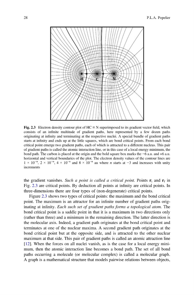
Figure 2.3 shows two types of critical points: the maximum and the bond critical
point. The maximum is an attractor for an infinite number of gradient paths originating at infinity. Each such set of gradient paths forms a topological atom. The
bond critical point is a saddle point in that it is a maximum in two directions only
(rather than three) and a minimum in the remaining direction. The latter direction is
the molecular axis. Indeed, a gradient path originates at the bond critical point and
terminates at one of the nuclear maxima. A second gradient path originates at the
bond critical point but at the opposite side, and is attracted to the other nuclear
maximum at that side. This pair of gradient paths is called an atomic attraction line
[12]. When the forces on all nuclei vanish, as is the case for a local energy minimum, then the atomic interaction line becomes a bond path. The set of all bond
paths occurring a molecule (or molecular complex) is called a molecular graph.
A graph is a mathematical structure that models pairwise relations between objects,
Fig. 2.3 Electron density contour plot of HC ≡ N superimposed to its gradient vector field, which
consists of an infinite multitude of gradient paths, here represented by a few dozen paths
originating at infinity and terminating at the respective nuclei. A special bundle of gradient paths
starts at infinity and ends up at the little squares, which are bond critical points. From each bond
critical point emerge two gradient paths, each of which is attracted to a different nucleus. This pair
of gradient paths is called the atomic interaction line, or in this case of a local energy minimum, the
bond path. The carbon is placed at the origin and the bold square box marks the −6 a.u. and +6 a.u.
horizontal and vertical boundaries of the plot. The electron density values of the contour lines are
1 × 10
−n
, 2 × 10
−n
, 4 × 10
−n and 8 × 10
−n au where n starts at −3 and increases with unity
increments
28
P.L.A. Popelier
Fig. 2.3 are critical points. By deduction all points at infinity are critical points. In
three-dimensions there are four types of (non-degenerate) critical points.
Figure 2.3 shows two types of critical points: the maximum and the bond critical
point. The maximum is an attractor for an infinite number of gradient paths originating at infinity. Each such set of gradient paths forms a topological atom. The
bond critical point is a saddle point in that it is a maximum in two directions only
(rather than three) and a minimum in the remaining direction. The latter direction is
the molecular axis. Indeed, a gradient path originates at the bond critical point and
terminates at one of the nuclear maxima. A second gradient path originates at the
bond critical point but at the opposite side, and is attracted to the other nuclear
maximum at that side. This pair of gradient paths is called an atomic attraction line
[12]. When the forces on all nuclei vanish, as is the case for a local energy minimum, then the atomic interaction line becomes a bond path. The set of all bond
paths occurring a molecule (or molecular complex) is called a molecular graph.
A graph is a mathematical structure that models pairwise relations between objects,
Fig. 2.3 Electron density contour plot of HC ≡ N superimposed to its gradient vector field, which
consists of an infinite multitude of gradient paths, here represented by a few dozen paths
originating at infinity and terminating at the respective nuclei. A special bundle of gradient paths
starts at infinity and ends up at the little squares, which are bond critical points. From each bond
critical point emerge two gradient paths, each of which is attracted to a different nucleus. This pair
of gradient paths is called the atomic interaction line, or in this case of a local energy minimum, the
bond path. The carbon is placed at the origin and the bold square box marks the −6 a.u. and +6 a.u.
horizontal and vertical boundaries of the plot. The electron density values of the contour lines are
1 × 10
−n
, 2 × 10
−n
, 4 × 10
−n and 8 × 10
−n au where n starts at −3 and increases with unity
increments
28
P.L.A. Popelier