

features. As a result, this difference density (technically known as the deformation
density) contains all the chemical features. Although a simple and innocent looking
approach, the exact form of the reference density is a concern. Different results can
be obtained for different choices made in constructing the deformation density.
However, there is a more minimal way forward, which avoids such choices in the
first place.
Occam’s razor proposes to use the molecular electron density as its own reference. Subtracting this density from itself returns a zero density everywhere, which
is of course useless but introducing the gradient achieves what is required. The
gradient represents an internal difference, via its definition as a derivative, which
contains the difference of two function values, each evaluated at two points
infinitesimally close to each other. At a given point, the gradient vector contains
local information on how the function (in the case the electron density) changes
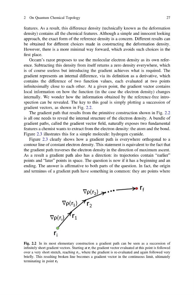
internally. We wonder how the information obtained by the reference-free introspection can be revealed. The key to this goal is simply plotting a succession of
gradient vectors, as shown in Fig. 2.2.
The gradient path that results from the primitive construction shown in Fig. 2.2
is all one needs to reveal the internal structure of the electron density. A bundle of
gradient paths, called the gradient vector field, naturally exposes two fundamental
features a chemist wants to extract from the electron density: the atom and the bond.
Figure 2.3 illustrates this for a simple molecule: hydrogen cyanide.
Figure 2.3 clearly shows how a gradient path is everywhere orthogonal to a
contour line of constant electron density. This statement is equivalent to the fact that
the gradient path traverses the electron density in the direction of maximum ascent.
As a result a gradient path also has a direction: its trajectories contain “earlier”
points and “later” points in space. The question is now if it has a beginning and an
ending. The answer is affirmative to both parts of the question. In fact, the origin
and terminus of a gradient path have something in common: they are points where
Fig. 2.2 In its most elementary construction a gradient path can be seen as a succession of
infinitely short gradient vectors. Starting at r i the gradient vector evaluated at this point is followed
over a very short stretch, reaching r 1 , where the gradient is re-evaluated and again followed very
briefly. This resulting broken line becomes a gradient vector in the continuous limit, ultimately
terminating in point r f
2 On Quantum Chemical Topology
27
density) contains all the chemical features. Although a simple and innocent looking
approach, the exact form of the reference density is a concern. Different results can
be obtained for different choices made in constructing the deformation density.
However, there is a more minimal way forward, which avoids such choices in the
first place.
Occam’s razor proposes to use the molecular electron density as its own reference. Subtracting this density from itself returns a zero density everywhere, which
is of course useless but introducing the gradient achieves what is required. The
gradient represents an internal difference, via its definition as a derivative, which
contains the difference of two function values, each evaluated at two points
infinitesimally close to each other. At a given point, the gradient vector contains
local information on how the function (in the case the electron density) changes
internally. We wonder how the information obtained by the reference-free introspection can be revealed. The key to this goal is simply plotting a succession of
gradient vectors, as shown in Fig. 2.2.
The gradient path that results from the primitive construction shown in Fig. 2.2
is all one needs to reveal the internal structure of the electron density. A bundle of
gradient paths, called the gradient vector field, naturally exposes two fundamental
features a chemist wants to extract from the electron density: the atom and the bond.
Figure 2.3 illustrates this for a simple molecule: hydrogen cyanide.
Figure 2.3 clearly shows how a gradient path is everywhere orthogonal to a
contour line of constant electron density. This statement is equivalent to the fact that
the gradient path traverses the electron density in the direction of maximum ascent.
As a result a gradient path also has a direction: its trajectories contain “earlier”
points and “later” points in space. The question is now if it has a beginning and an
ending. The answer is affirmative to both parts of the question. In fact, the origin
and terminus of a gradient path have something in common: they are points where
Fig. 2.2 In its most elementary construction a gradient path can be seen as a succession of
infinitely short gradient vectors. Starting at r i the gradient vector evaluated at this point is followed
over a very short stretch, reaching r 1 , where the gradient is re-evaluated and again followed very
briefly. This resulting broken line becomes a gradient vector in the continuous limit, ultimately
terminating in point r f
2 On Quantum Chemical Topology
27