

443
13 Continuous Molecular Fields Approach Applied to Structure-Activity Modeling
in Table 13.2. The training sets were used for building 3D-QSAR models and for
assessing their internal predictive performance using the 10-fold cross-validation
procedure. The test sets were used for assessing the external predictive performance
of the models.
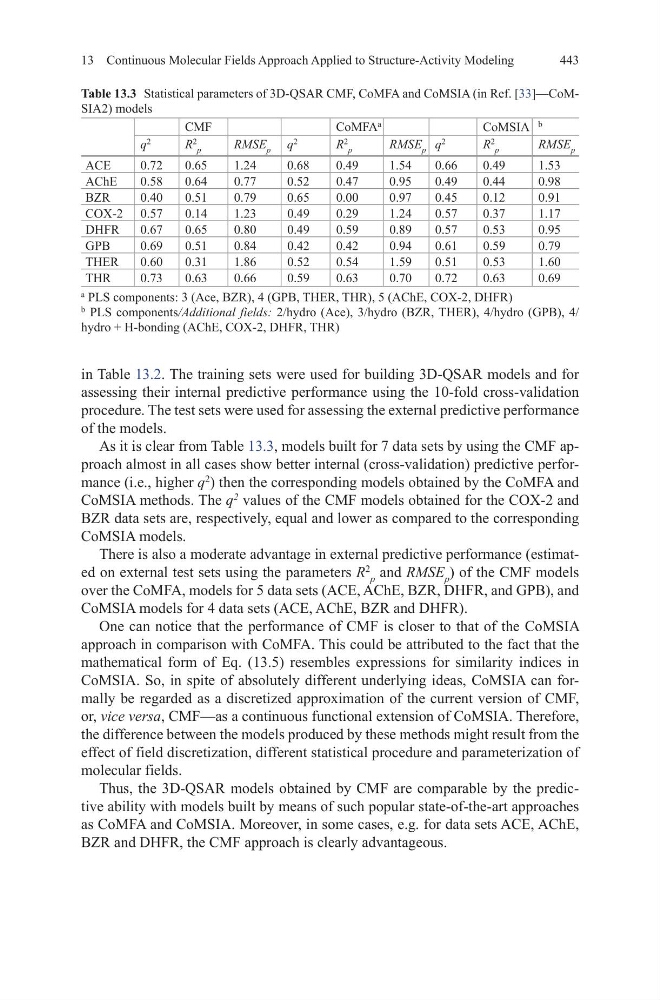
As it is clear from Table 13.3, models built for 7 data sets by using the CMF approach almost in all cases show better internal (cross-validation) predictive performance (i.e., higher q
2
) then the corresponding models obtained by the CoMFA and
CoMSIA methods. The q
2
values of the CMF models obtained for the COX-2 and
BZR data sets are, respectively, equal and lower as compared to the corresponding
CoMSIA models.
There is also a moderate advantage in external predictive performance (estimated on external test sets using the parameters R
2 p
and RMSE p ) of the CMF models
over the CoMFA, models for 5 data sets (ACE, AСhE, BZR, DHFR, and GPB), and
CoMSIA models for 4 data sets (ACE, AChE, BZR and DHFR).
One can notice that the performance of CMF is closer to that of the CoMSIA
approach in comparison with CoMFA. This could be attributed to the fact that the
mathematical form of Eq. (13.5) resembles expressions for similarity indices in
CoMSIA. So, in spite of absolutely different underlying ideas, CoMSIA can formally be regarded as a discretized approximation of the current version of CMF,
or, vice versa, CMF—as a continuous functional extension of CoMSIA. Therefore,
the difference between the models produced by these methods might result from the
effect of field discretization, different statistical procedure and parameterization of
molecular fields.
Thus, the 3D-QSAR models obtained by CMF are comparable by the predictive ability with models built by means of such popular state-of-the-art approaches
as CoMFA and CoMSIA. Moreover, in some cases, e.g. for data sets ACE, AChE,
BZR and DHFR, the CMF approach is clearly advantageous.
Table 13.3 Statistical parameters of 3D-QSAR CMF, CoMFA and CoMSIA (in Ref. [33]—CoMSIA2) models
CMF
CoMFA
a
CoMSIA
b
q
2
R
2 p
RMSE p q
2
R
2 p
RMSE p q
2
R
2 p
RMSE p
ACE
0.72
0.65
1.24
0.68
0.49
1.54
0.66
0.49
1.53
AChE
0.58
0.64
0.77
0.52
0.47
0.95
0.49
0.44
0.98
BZR
0.40
0.51
0.79
0.65
0.00
0.97
0.45
0.12
0.91
COX-2 0.57
0.14
1.23
0.49
0.29
1.24
0.57
0.37
1.17
DHFR
0.67
0.65
0.80
0.49
0.59
0.89
0.57
0.53
0.95
GPB
0.69
0.51
0.84
0.42
0.42
0.94
0.61
0.59
0.79
THER
0.60
0.31
1.86
0.52
0.54
1.59
0.51
0.53
1.60
THR
0.73
0.63
0.66
0.59
0.63
0.70
0.72
0.63
0.69
a
PLS components: 3 (Ace, BZR), 4 (GPB, THER, THR), 5 (AChE, COX-2, DHFR)
b
PLS components/Additional fields: 2/hydro (Ace), 3/hydro (BZR, THER), 4/hydro (GPB), 4/
hydro + H-bonding (AChE, COX-2, DHFR, THR)
13 Continuous Molecular Fields Approach Applied to Structure-Activity Modeling
in Table 13.2. The training sets were used for building 3D-QSAR models and for
assessing their internal predictive performance using the 10-fold cross-validation
procedure. The test sets were used for assessing the external predictive performance
of the models.
As it is clear from Table 13.3, models built for 7 data sets by using the CMF approach almost in all cases show better internal (cross-validation) predictive performance (i.e., higher q
2
) then the corresponding models obtained by the CoMFA and
CoMSIA methods. The q
2
values of the CMF models obtained for the COX-2 and
BZR data sets are, respectively, equal and lower as compared to the corresponding
CoMSIA models.
There is also a moderate advantage in external predictive performance (estimated on external test sets using the parameters R
2 p
and RMSE p ) of the CMF models
over the CoMFA, models for 5 data sets (ACE, AСhE, BZR, DHFR, and GPB), and
CoMSIA models for 4 data sets (ACE, AChE, BZR and DHFR).
One can notice that the performance of CMF is closer to that of the CoMSIA
approach in comparison with CoMFA. This could be attributed to the fact that the
mathematical form of Eq. (13.5) resembles expressions for similarity indices in
CoMSIA. So, in spite of absolutely different underlying ideas, CoMSIA can formally be regarded as a discretized approximation of the current version of CMF,
or, vice versa, CMF—as a continuous functional extension of CoMSIA. Therefore,
the difference between the models produced by these methods might result from the
effect of field discretization, different statistical procedure and parameterization of
molecular fields.
Thus, the 3D-QSAR models obtained by CMF are comparable by the predictive ability with models built by means of such popular state-of-the-art approaches
as CoMFA and CoMSIA. Moreover, in some cases, e.g. for data sets ACE, AChE,
BZR and DHFR, the CMF approach is clearly advantageous.
Table 13.3 Statistical parameters of 3D-QSAR CMF, CoMFA and CoMSIA (in Ref. [33]—CoMSIA2) models
CMF
CoMFA
a
CoMSIA
b
q
2
R
2 p
RMSE p q
2
R
2 p
RMSE p q
2
R
2 p
RMSE p
ACE
0.72
0.65
1.24
0.68
0.49
1.54
0.66
0.49
1.53
AChE
0.58
0.64
0.77
0.52
0.47
0.95
0.49
0.44
0.98
BZR
0.40
0.51
0.79
0.65
0.00
0.97
0.45
0.12
0.91
COX-2 0.57
0.14
1.23
0.49
0.29
1.24
0.57
0.37
1.17
DHFR
0.67
0.65
0.80
0.49
0.59
0.89
0.57
0.53
0.95
GPB
0.69
0.51
0.84
0.42
0.42
0.94
0.61
0.59
0.79
THER
0.60
0.31
1.86
0.52
0.54
1.59
0.51
0.53
1.60
THR
0.73
0.63
0.66
0.59
0.63
0.70
0.72
0.63
0.69
a
PLS components: 3 (Ace, BZR), 4 (GPB, THER, THR), 5 (AChE, COX-2, DHFR)
b
PLS components/Additional fields: 2/hydro (Ace), 3/hydro (BZR, THER), 4/hydro (GPB), 4/
hydro + H-bonding (AChE, COX-2, DHFR, THR)