

438
I. I. Baskin and N. I. Zhokhova
approximating continuous molecular fields. This provides the ability to use complex types of molecular fields, including those derived from quantum chemistry,
such as electron density functions.
13.2.2 The Use of Continuous Molecular Fields in Conjunction
with Regression Kernel-based Machine Learning Methods
Kernel K( M i, M j ), or its normalized version K’( M i, M j ), can be plugged in any kernelbased machine learning method (such as Support Vector Machine, Kernel Ridge
Regression [10], Kernel Partial Least Squares [28], Gaussian Processes, etc.) in
order to build regression, classification, novelty detection models, etc.
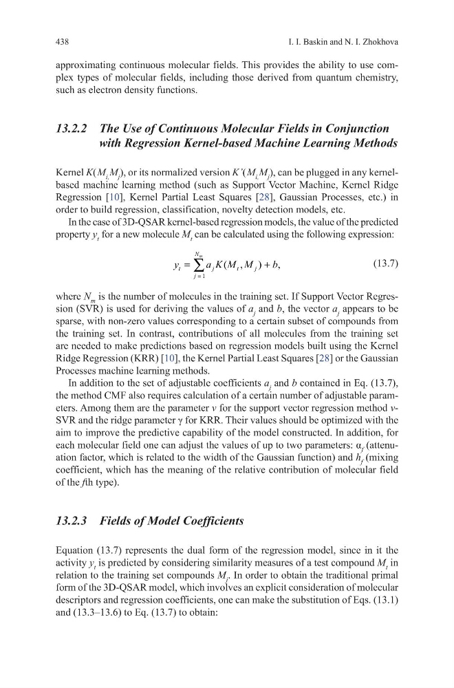
In the case of 3D-QSAR kernel-based regression models, the value of the predicted
property y t for a new molecule M t can be calculated using the following expression:
(13.7)
where N m is the number of molecules in the training set. If Support Vector Regression (SVR) is used for deriving the values of a j and b, the vector a j appears to be
sparse, with non-zero values corresponding to a certain subset of compounds from
the training set. In contrast, contributions of all molecules from the training set
are needed to make predictions based on regression models built using the Kernel
Ridge Regression (KRR) [10], the Kernel Partial Least Squares [28] or the Gaussian
Processes machine learning methods.
In addition to the set of adjustable coefficients a j and b contained in Eq. (13.7),
the method CMF also requires calculation of a certain number of adjustable parameters. Among them are the parameter v for the support vector regression method νSVR and the ridge parameter γ for KRR. Their values should be optimized with the
aim to improve the predictive capability of the model constructed. In addition, for
each molecular field one can adjust the values of up to two parameters: α f (attenuation factor, which is related to the width of the Gaussian function) and h f (mixing
coefficient, which has the meaning of the relative contribution of molecular field
of the fth type).
13.2.3 Fields of Model Coefficients
Equation (13.7) represents the dual form of the regression model, since in it the
activity y t is predicted by considering similarity measures of a test compound M t in
relation to the training set compounds M j . In order to obtain the traditional primal
form of the 3D-QSAR model, which involves an explicit consideration of molecular
descriptors and regression coefficients, one can make the substitution of Eqs. (13.1)
and (13.3–13.6) to Eq. (13.7) to obtain:
1
( ,
)
,
m
N
t
j
t
j
j
y
a K M M
b
=
=
+
∑
I. I. Baskin and N. I. Zhokhova
approximating continuous molecular fields. This provides the ability to use complex types of molecular fields, including those derived from quantum chemistry,
such as electron density functions.
13.2.2 The Use of Continuous Molecular Fields in Conjunction
with Regression Kernel-based Machine Learning Methods
Kernel K( M i, M j ), or its normalized version K’( M i, M j ), can be plugged in any kernelbased machine learning method (such as Support Vector Machine, Kernel Ridge
Regression [10], Kernel Partial Least Squares [28], Gaussian Processes, etc.) in
order to build regression, classification, novelty detection models, etc.
In the case of 3D-QSAR kernel-based regression models, the value of the predicted
property y t for a new molecule M t can be calculated using the following expression:
(13.7)
where N m is the number of molecules in the training set. If Support Vector Regression (SVR) is used for deriving the values of a j and b, the vector a j appears to be
sparse, with non-zero values corresponding to a certain subset of compounds from
the training set. In contrast, contributions of all molecules from the training set
are needed to make predictions based on regression models built using the Kernel
Ridge Regression (KRR) [10], the Kernel Partial Least Squares [28] or the Gaussian
Processes machine learning methods.
In addition to the set of adjustable coefficients a j and b contained in Eq. (13.7),
the method CMF also requires calculation of a certain number of adjustable parameters. Among them are the parameter v for the support vector regression method νSVR and the ridge parameter γ for KRR. Their values should be optimized with the
aim to improve the predictive capability of the model constructed. In addition, for
each molecular field one can adjust the values of up to two parameters: α f (attenuation factor, which is related to the width of the Gaussian function) and h f (mixing
coefficient, which has the meaning of the relative contribution of molecular field
of the fth type).
13.2.3 Fields of Model Coefficients
Equation (13.7) represents the dual form of the regression model, since in it the
activity y t is predicted by considering similarity measures of a test compound M t in
relation to the training set compounds M j . In order to obtain the traditional primal
form of the 3D-QSAR model, which involves an explicit consideration of molecular
descriptors and regression coefficients, one can make the substitution of Eqs. (13.1)
and (13.3–13.6) to Eq. (13.7) to obtain:
1
( ,
)
,
m
N
t
j
t
j
j
y
a K M M
b
=
=
+
∑