

437
13 Continuous Molecular Fields Approach Applied to Structure-Activity Modeling
(13.3)
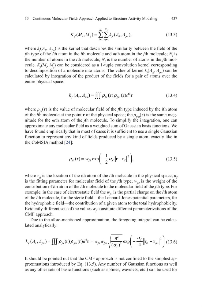
where k f ( A il , A jm ) is the kernel that describes the similarity between the field of the
fth type of the lth atom in the ith molecule and mth atom in the jth molecule; N i is
the number of atoms in the ith molecule; N j is the number of atoms in the jth molecule. K f (M i , M j ) can be considered as a 1-tuple convolution kernel corresponding
to decomposition of a molecule into atoms. The value of kernel k f ( A il , A jm ) can be
calculated by integration of the product of the fields for a pair of atoms over the
entire physical space:
(13.4)
where ρ fil (r) is the value of molecular field of the fth type induced by the lth atom
of the ith molecule at the point r of the physical space; the ρ fjm (r) is the same magnitude for the mth atom of the jth molecule. To simplify the integration, one can
approximate any molecular field as a weighted sum of Gaussian basis functions. We
have found empirically that in most of cases it is sufficient to use a single Gaussian
function to represent any kind of fields produced by a single atom, exactly like in
the CoMSIA method [24]:
(13.5)
where r il is the location of the lth atom of the ith molecule in the physical space; α f
is the fitting parameter for molecular field of the fth type; w fil is the weight of the
contribution of lth atom of the ith molecule to the molecular field of the fth type. For
example, in the case of electrostatic field the w fil is the partial charge on the lth atom
of the ith molecule, for the steric field—the Lennard-Jones potential parameters, for
the hydrophobic field—the contribution of a given atom to the total hydrophobicity.
Evidently different sets of the values w f constitute different parameterizations of the
CMF approach.
Due to the afore-mentioned approximation, the foregoing integral can be calculated analytically:
(13.6)
It should be pointed out that the CMF approach is not confined to the simplest approximations introduced by Eq. (13.5). Any number of Gaussian functions as well
as any other sets of basic functions (such as splines, wavelets, etc.) can be used for
1
1
( ,
)
( ,
),
j
i
N
N
f
i
j
f
il
jm
l
m
K M M
k A A
=
=
= ∑∑
3
( ,
)
( )
( )
f
il
jm
fil
fjm
k A A
d
ρ
ρ
= ∫∫∫ r
r r
2
1
( )
exp
,
2
fil
fil
f
il
w
ρ
α
=
-
-
r
r r
3
2
3
3
( ,
)
( )
( )
exp
4
( )
f
f
il
jm
fil
fjm
fil fjm
il
jm
f
k A A
d
w w
α
π
ρ
ρ
α
=
=
-
-
∫∫∫ r
r r
r r
13 Continuous Molecular Fields Approach Applied to Structure-Activity Modeling
(13.3)
where k f ( A il , A jm ) is the kernel that describes the similarity between the field of the
fth type of the lth atom in the ith molecule and mth atom in the jth molecule; N i is
the number of atoms in the ith molecule; N j is the number of atoms in the jth molecule. K f (M i , M j ) can be considered as a 1-tuple convolution kernel corresponding
to decomposition of a molecule into atoms. The value of kernel k f ( A il , A jm ) can be
calculated by integration of the product of the fields for a pair of atoms over the
entire physical space:
(13.4)
where ρ fil (r) is the value of molecular field of the fth type induced by the lth atom
of the ith molecule at the point r of the physical space; the ρ fjm (r) is the same magnitude for the mth atom of the jth molecule. To simplify the integration, one can
approximate any molecular field as a weighted sum of Gaussian basis functions. We
have found empirically that in most of cases it is sufficient to use a single Gaussian
function to represent any kind of fields produced by a single atom, exactly like in
the CoMSIA method [24]:
(13.5)
where r il is the location of the lth atom of the ith molecule in the physical space; α f
is the fitting parameter for molecular field of the fth type; w fil is the weight of the
contribution of lth atom of the ith molecule to the molecular field of the fth type. For
example, in the case of electrostatic field the w fil is the partial charge on the lth atom
of the ith molecule, for the steric field—the Lennard-Jones potential parameters, for
the hydrophobic field—the contribution of a given atom to the total hydrophobicity.
Evidently different sets of the values w f constitute different parameterizations of the
CMF approach.
Due to the afore-mentioned approximation, the foregoing integral can be calculated analytically:
(13.6)
It should be pointed out that the CMF approach is not confined to the simplest approximations introduced by Eq. (13.5). Any number of Gaussian functions as well
as any other sets of basic functions (such as splines, wavelets, etc.) can be used for
1
1
( ,
)
( ,
),
j
i
N
N
f
i
j
f
il
jm
l
m
K M M
k A A
=
=
= ∑∑
3
( ,
)
( )
( )
f
il
jm
fil
fjm
k A A
d
ρ
ρ
= ∫∫∫ r
r r
2
1
( )
exp
,
2
fil
fil
f
il
w
ρ
α
=
-
-
r
r r
3
2
3
3
( ,
)
( )
( )
exp
4
( )
f
f
il
jm
fil
fjm
fil fjm
il
jm
f
k A A
d
w w
α
π
ρ
ρ
α
=
=
-
-
∫∫∫ r
r r
r r