

436
I. I. Baskin and N. I. Zhokhova
of grids is very high dimensionality of the regression task caused by the big number
of grid points, which precludes the use of many efficient statistical methods. Unfortunately, decrease of the number of grid points through increase of the step size
(i.e. the use of coarser grid) or decrease of its extent causes the loss of important
information. In order to tackle the problem, we suggest not using grids or fixed
probe positions in 3D-QSAR studies. Instead of computing descriptor values at a
discrete set of points, we propose to work directly with descriptions of molecular
fields in the form of continuous functions on radius vector r, by means of specially
constructed kernels. The use of such continuous molecular fields seems to be much
more natural and corresponding to the real physical picture of the world than the
application of certain speculative grids arbitrary chosen to approximate such fields.
It should be mentioned that continuous molecular fields have already been used
in QSAR studies. So, indexes of R. Carbó-Dorca, which were used in certain QSAR
studies [27], can also be considered as a particular case of continuous molecular
fields.
The method of Continuous Molecular Fields (CMF) performs statistical analysis
of functional molecular data by means of joint application of kernel machine learning methods and special kernels which compare molecules by computing overlap
integrals of their molecular fields [7, 8].
13.2.1 Procedure of Kernel Calculation
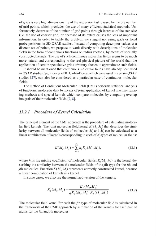
The principal element of the CMF approach is the procedure of calculating molecular field kernels. The joint molecular field kernel K( M i , M j ) that describes the similarity between all molecular fields of molecules M i and M j can be calculated as a
linear combination of kernels corresponding to each of N f types of molecular fields:
(13.1)
where h f is the mixing coefficient of molecular fields; K f (M i , M j ) is the kernel describing the similarity between the molecular fields of the fth type for the ith and
jth molecules. Function K( M i , M j ) represents correctly constructed kernel, because
a linear combination of kernels is a kernel.
In some cases, we also use the normalized version of the kernels:
(13.2)
The molecular field kernel for each the fth type of molecular field is calculated in
the framework of the CMF approach by summation of the kernels for each pair of
atoms for the ith and jth molecules:
K M M
h K M M
i
j
f
f
i
j
f
N f
( ,
)
( ,
),
=
=
∑
1
'
( , )
( , )
( , )
( , )
f
i
j
f
i
j
f
i
i
f
j
j
K M M
K M M
K M M K M M
=
⋅
I. I. Baskin and N. I. Zhokhova
of grids is very high dimensionality of the regression task caused by the big number
of grid points, which precludes the use of many efficient statistical methods. Unfortunately, decrease of the number of grid points through increase of the step size
(i.e. the use of coarser grid) or decrease of its extent causes the loss of important
information. In order to tackle the problem, we suggest not using grids or fixed
probe positions in 3D-QSAR studies. Instead of computing descriptor values at a
discrete set of points, we propose to work directly with descriptions of molecular
fields in the form of continuous functions on radius vector r, by means of specially
constructed kernels. The use of such continuous molecular fields seems to be much
more natural and corresponding to the real physical picture of the world than the
application of certain speculative grids arbitrary chosen to approximate such fields.
It should be mentioned that continuous molecular fields have already been used
in QSAR studies. So, indexes of R. Carbó-Dorca, which were used in certain QSAR
studies [27], can also be considered as a particular case of continuous molecular
fields.
The method of Continuous Molecular Fields (CMF) performs statistical analysis
of functional molecular data by means of joint application of kernel machine learning methods and special kernels which compare molecules by computing overlap
integrals of their molecular fields [7, 8].
13.2.1 Procedure of Kernel Calculation
The principal element of the CMF approach is the procedure of calculating molecular field kernels. The joint molecular field kernel K( M i , M j ) that describes the similarity between all molecular fields of molecules M i and M j can be calculated as a
linear combination of kernels corresponding to each of N f types of molecular fields:
(13.1)
where h f is the mixing coefficient of molecular fields; K f (M i , M j ) is the kernel describing the similarity between the molecular fields of the fth type for the ith and
jth molecules. Function K( M i , M j ) represents correctly constructed kernel, because
a linear combination of kernels is a kernel.
In some cases, we also use the normalized version of the kernels:
(13.2)
The molecular field kernel for each the fth type of molecular field is calculated in
the framework of the CMF approach by summation of the kernels for each pair of
atoms for the ith and jth molecules:
K M M
h K M M
i
j
f
f
i
j
f
N f
( ,
)
( ,
),
=
=
∑
1
'
( , )
( , )
( , )
( , )
f
i
j
f
i
j
f
i
i
f
j
j
K M M
K M M
K M M K M M
=
⋅